
A pivot table summarises a list of rows into a grouped cross-tabulation. You drag field names into four zones and Excel calculates the totals, counts, or averages for every combination. The layout is live: drag a field out, drag another in, and the numbers rebuild instantly without touching the source data.
This guide covers the full build process for Excel and Google Sheets, plus date grouping, slicers, calculated fields, and the most common fixes. It belongs to our Excel category. Use the Pivot Table Maker if you want to build one from your own data right now.
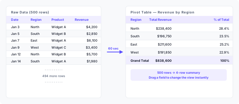
| Region | Total Revenue | % of Total |
|---|---|---|
| North | $238,400 | 28.4% |
| South | $196,750 | 23.5% |
| East | $211,600 | 25.2% |
| West | $191,850 | 22.9% |
| Total | $838,600 | 100% |
This four-row summary came from 500 rows of raw sales data. Each row in the pivot table is a region. Its Revenue cell is the sum of every source row that shares that region label. Start by checking what one source row represents.
What does a pivot table contain?
Four zones control the layout. Each column header from your source data can go into one or more of them.
| Zone | What it does | Example field |
|---|---|---|
| Rows | Creates one row per unique value of this field | Region |
| Columns | Creates one column per unique value of this field | Quarter |
| Values | Aggregates a numeric field — sum, count, or average | Revenue |
| Filters | Filters the whole table to a chosen subset of values | Salesperson |
A field in Rows becomes the row labels on the left side of the table. A field in Values gets aggregated — the default aggregation is SUM for numbers and COUNT for text. You can place multiple fields in the same zone, and the same field can appear in both Rows and Values at the same time.
What your source data needs
| Requirement | Why it matters |
|---|---|
| One row per observation | Each row is one transaction, response, or record — not a subtotal |
| Column headers in row 1 | Excel uses these as field names in the Fields pane |
| No blank rows or columns | Excel stops detecting the range at the first blank row |
| No merged cells | Merged cells create blank cells that break row grouping |
| Consistent date formats | Mixed formats prevent date grouping from working |
| Numbers stored as numbers | Numbers stored as text are counted, not summed |
Fix these issues before inserting the pivot table. Fixing them afterwards requires deleting and rebuilding the table from scratch.
How to make a pivot table in Excel
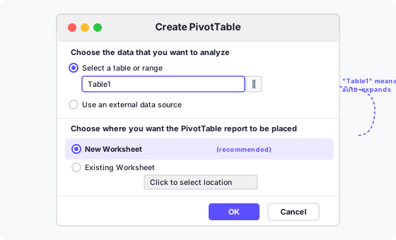
- Select any cell in your data. Excel detects the full range automatically, stopping at the first blank row or column.
- Insert → PivotTable. On the ribbon choose Insert, then PivotTable. The keyboard path is Alt → N → V → T (press each key in sequence, not together).
- Confirm the range. Excel highlights the detected range with a dashed border. If it looks wrong, correct it in the Table/Range box. Leave New Worksheet selected and click OK.
- Drag a field to Rows. In the Fields pane on the right, drag Region into the Rows area at the bottom. One row appears per unique region.
- Drag a field to Values. Drag Revenue into the Values area. Excel fills each row with the sum of Revenue for that region.
- Check the totals. The Grand Total row at the bottom should equal the sum of your entire Revenue column. A mismatch points to a data quality issue in the source.
- Add more fields as needed. Drag Quarter to Columns to break revenue down by quarter. Drag Salesperson to Filters to add a dropdown that narrows the whole table.
- Refresh after data changes. Right-click anywhere inside the pivot table and choose Refresh, or press Alt+F5. The table reads the source range again and updates every cell.
Use the Pivot Table Maker to build your first summary from a CSV file without opening Excel.
Reading the Fields pane
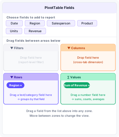
The upper half lists every column header from your source data as a draggable chip. The lower half shows the four zones. A chip in Rows or Columns shows in the zone without a prefix. A chip in Values shows as "Sum of Revenue" or "Count of Product" — Excel adds the aggregation function as a prefix automatically.
To change the aggregation, click the chip in the Values zone, choose Value Field Settings, and pick from Sum, Count, Average, Max, Min, or Product. You can add the same field to Values twice with two different aggregations: one copy showing Sum, another showing Average, in adjacent columns.
How to make a pivot table in Google Sheets
- Select any cell in your data.
- Insert → Pivot table. Choose whether to place it in a new sheet or the existing one.
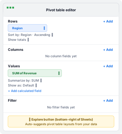
- Add Rows. In the pivot table editor on the right, click Add next to Rows and choose Region.
- Add Values. Click Add next to Values and choose Revenue. The editor defaults to SUM.
- Sort and filter. Use the Sort and Show totals options below each field in the editor panel to control ordering and subtotals.
The Explore button in the bottom-right corner of the Sheets window can suggest a pivot table layout automatically. It is a useful starting point, but check that it has picked the right aggregation for your question. Google Sheets pivot tables refresh automatically; there is no manual Refresh step.
Keep the pivot table up to date as data grows
By default, an Excel pivot table references a fixed range such as $A$1:$F$501. When you add row 502, it falls outside the range and the pivot table misses it.
Convert the source to an Excel Table first. Select any cell in your data and press Ctrl+T. Excel wraps the range in a named Table (Table1 by default) and extends it automatically whenever you add rows at the bottom. The pivot table's range reference then reads Table1 instead of a fixed address. After adding rows, still press Alt+F5 to refresh. The Table handles the range; the refresh handles the recalculation. Skipping the refresh leaves the pivot table showing stale totals even though the source is current.
Group dates by month or quarter
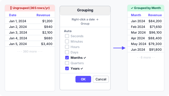
A date field in Rows without grouping creates one row for every unique date in the source — often hundreds of rows. Right-click any date cell in the pivot table and choose Group to open the Grouping dialog.
Select Months and Years together. Selecting Years alone gives one row per year. Selecting Months alone collapses all Januaries regardless of year into a single "Jan" row. With both selected, each row shows a distinct month-year pair such as Jan 2024, Feb 2024.
Quarters are a third option. Select Quarters and Years to get Q1 2024, Q2 2024. You can select multiple groupings at once — the pivot table adds an expandable hierarchy with the coarser grouping on the outside.
If the Group option is greyed out, your date column contains at least one value Excel does not recognise as a date — often a blank cell or a text string such as "N/A". Fix those values in the source, refresh, and try again [2].
Add a calculated field
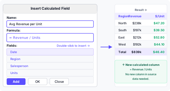
A calculated field creates a new Values column using a formula that refers to other fields by name. It is computed inside the pivot table, so the source data needs no new column.
To insert one: click anywhere in the pivot table, then go to PivotTable Analyze → Fields, Items & Sets → Calculated Field. Enter a name and a formula. Use field names as variables: = Revenue / Units divides the sum of Revenue by the sum of Units for each row.
The formula operates on aggregated values, not row-by-row values. = Revenue / Units gives total revenue divided by total units for a region — a weighted average. It does not calculate each row's unit price and then average those. For row-level calculations, add the formula column to the source data before creating the pivot table [1].
Show values as percentages
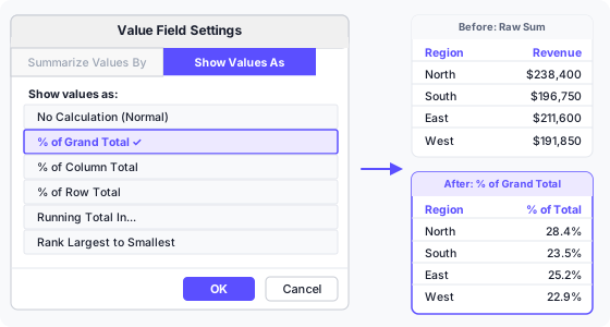
Right-click any cell in the Values column and choose Value Field Settings → Show Values As. Useful options:
| Option | Shows | Use when |
|---|---|---|
| % of Grand Total | Each cell as a share of the overall total | Comparing contributions across all rows and columns |
| % of Column Total | Each cell as a share of its column's subtotal | Comparing rows within each column independently |
| % of Row Total | Each cell as a share of its row's subtotal | Comparing columns within each row independently |
| Running Total In | Cumulative sum down the rows | Tracking progress toward a target over time |
| Rank Largest to Smallest | Rank number instead of value | Identifying the top-performing category quickly |
You can show both the raw sum and the percentage simultaneously by adding the Revenue field to Values twice — once set to Normal, once set to % of Grand Total. Click the chip in the Values zone a second time to add it again, then change only the second copy's Show Values As setting.
Filter with slicers
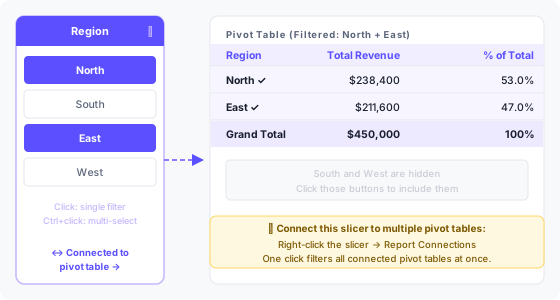
A slicer is a floating button panel that filters a pivot table visually. Click PivotTable Analyze → Insert Slicer, then choose the fields you want as filter buttons. Click a button to include that value. Hold Ctrl and click to select multiple values. Click the ✕ icon on the slicer to clear all filters.
One slicer can control multiple pivot tables at once. Right-click the slicer, choose Report Connections, then tick every pivot table in the workbook that should respond to it. This is useful for dashboards where several summaries share the same filter.
Timelines work the same way but are purpose-built for date fields. Insert one with PivotTable Analyze → Insert Timeline. It shows a horizontal bar grouped by months, quarters, or years that you drag to select a date range [3].
Pivot table versus SUMIF
| Situation | Pivot table | SUMIF / SUMIFS |
|---|---|---|
| Exploring unknown groupings | Yes — drag and drop to change | No — requires rewriting formulas |
| Output must update automatically | No — requires a manual refresh | Yes — recalculates with the sheet |
| Summary changes frequently | Yes — refresh once | No — may need new criteria columns |
| Fixed formula feeding another cell | Awkward — results shift if layout changes | Yes — reference is stable |
| Multiple criteria at once | Yes — Rows + Columns + Filters | Yes — SUMIFS handles up to 127 criteria ranges |
Use a pivot table when you are exploring the data or when the groupings change. Use SUMIF when the output feeds another formula or the layout is fixed and must update without user interaction.
Common problems and fixes
- Values show Count instead of Sum. The field contains at least one blank cell or a cell with text. Excel defaults to COUNT when it finds non-numeric data. Fix the source, delete the field from Values, and add it back.
- Group option is greyed out. The date column has mixed types — at least one cell is blank, text, or a number formatted to look like a date. Use Data → Text to Columns or filter for non-date values to find the offending cell.
- New rows are missing after refresh. The source range is a fixed address, not an Excel Table. Convert with Ctrl+T, then verify the pivot table's data source shows Table1 under PivotTable Analyze → Change Data Source.
- Grand Total does not match a manual SUM. A calculated field or a Show Values As setting is altering the total. Check both. You can also hide the Grand Total row under PivotTable Design → Grand Totals.
- Percentage column shows 100% for every row. Show Values As is set to % of Row Total instead of % of Grand Total. Right-click the Values column and change it.
- Filter dropdown shows deleted values. Excel remembers every value that ever appeared in a field. Go to PivotTable Options → Data → Number of items to retain per field, set it to None, then refresh.
- Date grouping creates an unwanted hierarchy. You selected multiple groupings (Months + Years) but want months only. Right-click the date cells → Ungroup, then re-open Grouping and select Months alone.
- Pivot table moves when source data expands. The pivot table is on the same sheet as the source. Place pivot tables on a separate sheet to avoid layout conflicts when new rows push data down.
Keyboard shortcuts
| Action | Keys |
|---|---|
| Insert pivot table | Alt → N → V → T |
| Refresh active pivot table | Alt+F5 |
| Refresh all pivot tables | Ctrl+Alt+F5 |
| Open Value Field Settings | Double-click any Values cell |
| Expand or collapse a row | Alt+Shift+= or - |
| Group selected items | Alt+Shift+→ |
| Ungroup selected items | Alt+Shift+← |
| Select entire pivot table | Ctrl+A (while inside the table) |
| Convert source to Excel Table | Ctrl+T |
| Open PivotTable Fields pane | Alt+J+T+L |
Frequently asked questions
What is a pivot table?
A pivot table groups and aggregates rows from a flat data table. You choose which fields label the rows and columns and which numeric field gets summed or counted. The result is a compact cross-tabulation that can be rearranged without touching the source data.
How do you make a pivot table in Excel?
Select any cell in your data, choose Insert → PivotTable, confirm the range, and click OK. In the Fields pane on the new sheet, drag a category field to Rows and a numeric field to Values. Excel fills in the totals immediately.
How do you make a pivot table in Google Sheets?
Select your data, choose Insert → Pivot table, pick the destination sheet, then use the editor panel on the right to add rows, columns, and values. Changes take effect immediately without a separate refresh step.
Why is my pivot table showing Count instead of Sum?
At least one cell in that column contains text or is blank. Excel counts non-numeric data instead of summing it. Fix those cells in the source, remove the field from Values, and add it back.
How do you refresh a pivot table?
Right-click anywhere in the pivot table and choose Refresh, or press Alt+F5. To refresh all pivot tables in the workbook at once, press Ctrl+Alt+F5. Google Sheets refreshes automatically whenever the source changes.
How do you add a calculated field to a pivot table?
Click anywhere in the pivot table, go to PivotTable Analyze → Fields, Items & Sets → Calculated Field. Enter a name and a formula using field names from your source data as variables. The result appears as a new column in the pivot table.
How do you group dates by month in a pivot table?
Right-click any date value in the Rows area and choose Group. In the Grouping dialog, select Months and Years together, then click OK. Each row will show a month-year pair such as Jan 2024, Feb 2024.
What is the difference between a slicer and a filter?
A filter is a dropdown inside the pivot table header that narrows by one field. A slicer is a separate floating panel with clickable buttons. Slicers show the active state at a glance, support multi-select with Ctrl+click, and can be connected to multiple pivot tables at once.
Can a pivot table update automatically when new data is added?
Not without a macro, but converting the source to an Excel Table with Ctrl+T ensures the range covers new rows the moment you refresh. The range expands automatically; only the refresh step remains manual.
What data format does a pivot table need?
One observation per row, column headers in row 1, no blank rows or columns, no merged cells, numbers stored as numbers, and dates in a format Excel recognises as a date. These are the minimum requirements before inserting.
References
- Microsoft Support: Calculated field and calculated item in a PivotTable
- Microsoft Support: Group or ungroup data in a PivotTable
- Microsoft Support: Use slicers to filter data