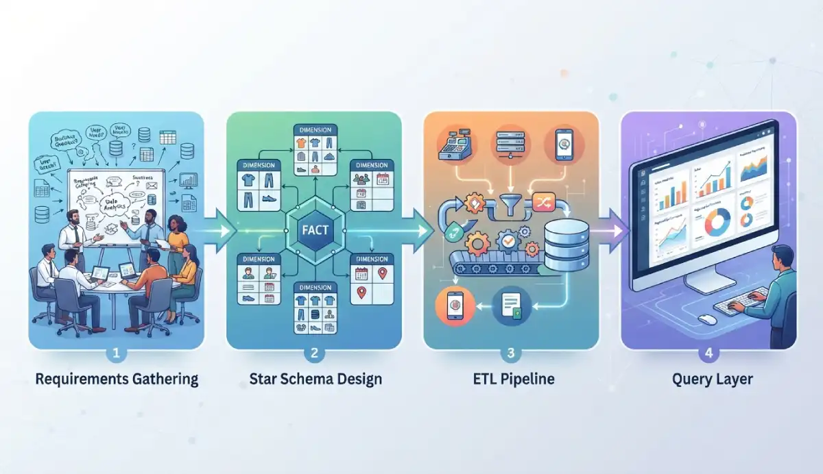
Most data warehouse projects are designed backwards. Teams pick a cloud platform first, build tables around it, write ETL to fill those tables, and then ask what the warehouse was supposed to answer. That sequence produces a technically sound system built for the wrong problem. The correct order is requirements, then schema, then ETL, then query layer — each phase depends on the output of the one before it. This guide walks all four with working SQL and a single running example: ClothCo, a clothing e-commerce company that needs to report on daily revenue by product, region, and customer segment. That business requirement starts as a note on paper in Phase 1 and ends as a 10-line SELECT in Phase 4. For the broader picture of how warehousing fits into analytical work, the data analysis overview covers the foundations before you go deep on warehouse architecture.
🛠 Mapping your schema? Use the Star Schema Designer → to lay out fact and dimension tables visually before writing any DDL.
📊 Making the case to leadership? Calculate your projected ROI with the DW ROI Calculator →
What Is a Data Warehouse? (And When Do You Need One?)
A data warehouse is a database built for reading, not writing. Your operational database — the one your app writes orders into — handles thousands of small writes per second. A warehouse handles a different job: a GROUP BY across three years of order data, joining five tables, returning in two seconds. Same underlying data, completely different architecture.
The technical distinction is OLTP versus OLAP. OLTP (Online Transaction Processing) is your production database: normalized schema, write-optimized, one row at a time. OLAP (Online Analytical Processing) is your warehouse: denormalized schema, read-optimized, millions of rows at a time. The same e-commerce order data that lives in a PostgreSQL production database gets restructured into a star schema in the warehouse so analytical queries run fast.
You need a data warehouse when:
- Analysts need to combine data from two or more source systems — CRM, e-commerce platform, ad accounts
- Ad hoc SQL queries against your production database are slowing it down or getting blocked by the DBA team
- Your team is joining data in spreadsheets because the production database is off-limits
- You need historical snapshots of data the operational system overwrites — like customer segments or product prices that change over time
You don't need a data warehouse when:
- One database already answers every business question your team has
- Your total data volume is under 10 GB and growing slowly
- No one on the team can maintain it after the initial build
The Four Phases of Building a Data Warehouse
The phases run in sequence. Teams that jump straight to tool selection — the most common mistake — spend months loading data nobody queries.

- Phase 1: Requirements Gathering — Define the business questions the warehouse must answer, inventory source systems, agree on the grain, set a 90-day scope
- Phase 2: Schema Design — Model your data as fact tables and dimension tables in a star schema
- Phase 3: ETL Pipeline — Extract data from sources, transform it to match the schema, load it into the warehouse on a schedule
- Phase 4: Query Layer — Build SQL views that pre-join the star schema tables and expose clean columns to BI tools
Phase 1 — Requirements Gathering
This is the phase most technical teams skip — and the reason most data warehouses fail. The goal is to answer four questions before writing a single line of SQL.
Question 1: What decisions will the warehouse enable? Start with the reports and dashboards the business actually needs, then work backwards. If the VP of Sales needs weekly revenue by product category and region, that determines your fact table (order line items), your dimensions (date, product, geography), and your grain (one row per order line). Start from the report, not from the source schema.
Question 2: Where does the data live today? List every source system: the transactional database (PostgreSQL, MySQL, SQL Server), the CRM (Salesforce, HubSpot), the e-commerce platform (Shopify), the ad platforms (Google, Meta). Note the update frequency — daily batch, hourly, near-real-time. This determines your ETL schedule in Phase 3.
Question 3: What is the data quality like? Audit source data before loading anything. Common problems: nulls in key fields, duplicate records, inconsistent date formats in the same column, and referential integrity gaps — order line items whose product IDs don't exist in the product table. Poor source data quality is the single biggest variable in how long ETL development takes. The exploratory data analysis guide covers auditing techniques you can run on source exports before the first table is designed.
Question 4: What does done look like in 90 days? Define a minimum viable warehouse: one business process (sales orders), three to five dimensions (date, product, customer, geography), and two dashboards. Data warehouse projects expand until they don't ship. Agree on scope in writing before the first table is designed.
Running Example — ClothCo Requirements
ClothCo sells clothing online, with transactions in PostgreSQL and customer data in HubSpot. Four questions drive the warehouse build:
| Business Question | Facts Needed | Dimensions Needed |
|---|---|---|
| Revenue by product category per week | sales_amount | dim_date, dim_product |
| Top customers by lifetime value | sales_amount, quantity | dim_customer |
| Regional performance comparison | sales_amount | dim_geography |
| Return rate by product | return_amount | dim_product, dim_date |
Grain decision: One row in the fact table equals one order line item — not one order, not one day's total. This is the finest granularity that answers all four questions without losing information. Write the grain as a SQL comment on the CREATE TABLE statement. When a new data engineer joins 18 months from now, they should not have to guess what a fact table row represents.
📐 Once you know your row count and grain, estimate storage costs before choosing a platform — use the Data Warehouse Sizing Calculator →
Phase 2 — Schema Design (Dimensional Modeling)
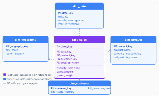
Schema design translates the requirements output — fact definitions, dimension lists, and grain — into actual database tables. The industry standard for analytical workloads is dimensional modeling, developed by Ralph Kimball and still the dominant approach for warehouses built today.
Dimensional modeling organizes data into two table types:
- Fact tables — Each row is one event at the defined grain. Columns are numeric measures (sales_amount, quantity_sold, gross_margin) plus integer foreign keys that point to each dimension table.
- Dimension tables — Each row describes one thing: a product, a customer, a date, a geography. Columns are descriptive attributes: product_name, category, color, size, segment, region.
The result is a star schema: the fact table sits at the center; dimension tables radiate outward. BI tools and analysts join the fact table to whichever dimensions they need. Because dimension tables are denormalized — no sub-tables, no normalization layers — joins are simple and query performance is fast.
Star Schema vs. Snowflake Schema — Decision Table
A snowflake schema normalizes the dimension tables further. In a snowflake, dim_product might break into dim_product and dim_category joined by a foreign key. This saves storage but adds query complexity. Here is when each schema makes sense:
| Criterion | Star Schema | Snowflake Schema |
|---|---|---|
| Query performance | ✓ Faster — fewer joins required | Slower — multi-hop joins for every query |
| Storage usage | Higher — denormalized values repeated | ✓ Lower — normalized, less repetition |
| SQL complexity for analysts | ✓ Simpler — direct dimension joins | More complex — joining through sub-dimensions |
| Dimension attribute updates | Update multiple rows | ✓ Update in one place |
| Use when | BI and analytics are the priority | Storage is tightly constrained and dimensions update frequently |
For ClothCo — and for most teams building a first warehouse — use star schema. Analyst productivity matters more than the marginal storage saving from normalization.
Kimball vs. Inmon — Which Methodology?

| Dimension | Kimball (Bottom-Up) | Inmon (Top-Down) |
|---|---|---|
| Starting point | One business process (e.g., sales orders) | Full enterprise data model in 3NF |
| Time to first value | Weeks | Months or years |
| Team size required | 1–5 people | 5–20+ people |
| Risk level | Lower — build incrementally, fix as you go | Higher — large upfront design investment |
| Output | Star schemas per subject area, expanded over time | Normalized 3NF EDW → subject-area data marts |
Recommendation for most teams: use Kimball. Build the sales star schema. Ship it in 4–6 weeks. Add the marketing star schema next quarter. The incremental approach means every mistake is fixable and every delivery proves value to stakeholders. Inmon is the right choice for large enterprises with dedicated data architecture teams and an 18-month project runway — not a two-person data team at a 200-person company.
🛠 Ready to design your schema? Map fact tables, dimension tables, and foreign key relationships visually with the Star Schema Designer → before writing DDL.
SQL — Creating the ClothCo Star Schema
Each dimension table gets an integer surrogate key — not the natural key from the source system. Source system IDs can change, be reused, or collide across systems when two sources are merged. Surrogate keys are stable integers generated by the warehouse, independent of anything upstream.
-- Dimension: Date
-- Populated once at build time; covers 10+ years of dates
CREATE TABLE dim_date (
    date_key        INT PRIMARY KEY,         -- surrogate key: YYYYMMDD format
    full_date       DATE NOT NULL,
    day_of_week     VARCHAR(10),
    week_number     INT,
    month_number    INT,
    month_name      VARCHAR(10),
    quarter         INT,
    year            INT,
    is_weekend      BOOLEAN
);

-- Dimension: Product
CREATE TABLE dim_product (
    product_key     INT PRIMARY KEY,
    product_id      VARCHAR(50),             -- natural key from source system
    product_name    VARCHAR(200) NOT NULL,
    category        VARCHAR(100),
    subcategory     VARCHAR(100),
    color           VARCHAR(50),
    size            VARCHAR(20),
    unit_cost       DECIMAL(10,2),
    is_current      BOOLEAN DEFAULT TRUE     -- for SCD Type 2 tracking
);

-- Dimension: Customer
CREATE TABLE dim_customer (
    customer_key    INT PRIMARY KEY,
    customer_id     VARCHAR(50),
    full_name       VARCHAR(200),
    email           VARCHAR(200),
    segment         VARCHAR(50),             -- e.g., 'VIP', 'Standard', 'New'
    city            VARCHAR(100),
    state           VARCHAR(100),
    country         VARCHAR(100)
);

-- Dimension: Geography
CREATE TABLE dim_geography (
    geography_key   INT PRIMARY KEY,
    city            VARCHAR(100),
    state           VARCHAR(100),
    region          VARCHAR(50),             -- e.g., 'Northeast', 'West'
    country         VARCHAR(100)
);

-- Fact: Sales
-- Grain: one row per order line item
CREATE TABLE fact_sales (
    sales_key       BIGINT PRIMARY KEY,
    order_id        VARCHAR(50) NOT NULL,    -- natural key from source
    date_key        INT REFERENCES dim_date(date_key),
    product_key     INT REFERENCES dim_product(product_key),
    customer_key    INT REFERENCES dim_customer(customer_key),
    geography_key   INT REFERENCES dim_geography(geography_key),
    quantity        INT NOT NULL,
    unit_price      DECIMAL(10,2) NOT NULL,
    discount_amount DECIMAL(10,2) DEFAULT 0,
    sales_amount    DECIMAL(10,2) NOT NULL,  -- (unit_price * quantity) - discount
    cost_amount     DECIMAL(10,2),
    gross_margin    DECIMAL(10,2)            -- sales_amount - cost_amount
);
🔍 Paste this DDL into the SQL Schema Visualizer → to generate an ER diagram of your star schema automatically.
Phase 3 — Building the ETL Pipeline
ETL (Extract, Transform, Load) moves data from source systems into the warehouse schema on a schedule. The pipeline runs through three distinct layers, each with a different job.
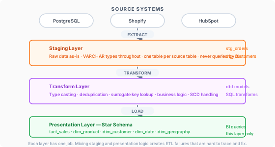
- Staging layer — Raw data, unchanged, lands here first. One staging table per source system table. No transformations. This layer exists to protect the presentation layer from upstream schema changes — if a source column is renamed, staging catches it before the fact table breaks.
- Transform layer — Cleanse, deduplicate, type-cast, derive new columns, resolve surrogate keys, apply business logic. This is where your rules live.
- Presentation layer — The final star schema tables: fact_sales, dim_product, dim_customer, and so on. BI tools only ever query this layer.
ETL vs. ELT: the difference is where transformation happens.
| Approach | Transform before or after loading? | Best for |
|---|---|---|
| ETL | Transform BEFORE loading into the warehouse | Traditional on-premises systems; sensitive data that must not land raw |
| ELT | Load raw FIRST, then transform inside the warehouse | Cloud warehouses (Snowflake, BigQuery, Redshift) with enough compute for in-database transformation |
Modern cloud warehouses have more than enough compute to transform inside the database. Load raw data fast with Fivetran or Airbyte, then write your transformation logic in SQL using dbt. The ELT pattern is faster to implement than traditional ETL tools and version-controls the transformation logic in git alongside your schema DDL.
SQL — Staging Layer for ClothCo
The staging table mirrors the source orders table with raw VARCHAR types throughout. No casting, no cleaning — just land the data.
-- Staging table mirrors the source system orders table
-- Raw VARCHAR types throughout — transformation happens downstream
CREATE TABLE stg_orders (
    raw_id          BIGINT PRIMARY KEY,
    source_order_id VARCHAR(50),
    order_date      VARCHAR(30),             -- raw string; transform layer handles type casting
    customer_id     VARCHAR(50),
    product_id      VARCHAR(50),
    qty             VARCHAR(20),             -- may arrive as string from API responses
    price           VARCHAR(20),
    discount        VARCHAR(20),
    city            VARCHAR(100),
    country         VARCHAR(100),
    loaded_at       TIMESTAMP DEFAULT NOW()
);
SQL — Loading the Fact Table from Staging
This INSERT joins four dimension tables to resolve surrogate keys, casts raw VARCHAR columns to their target types, and calculates derived measures. The WHERE NOT EXISTS clause handles incremental loading — rows already in the fact table are skipped on each run.
-- Insert new order lines into fact_sales from staged data
-- Joins to dimensions to resolve surrogate keys
INSERT INTO fact_sales (
    order_id, date_key, product_key, customer_key, geography_key,
    quantity, unit_price, discount_amount, sales_amount, cost_amount, gross_margin
)
SELECT
    s.source_order_id,
    d.date_key,
    p.product_key,
    c.customer_key,
    g.geography_key,
    CAST(s.qty AS INT),
    CAST(s.price AS DECIMAL(10,2)),
    COALESCE(CAST(s.discount AS DECIMAL(10,2)), 0),
    -- sales_amount = (price x qty) minus discount
    (CAST(s.price AS DECIMAL(10,2)) * CAST(s.qty AS INT))
        - COALESCE(CAST(s.discount AS DECIMAL(10,2)), 0),
    p.unit_cost * CAST(s.qty AS INT),
    -- gross_margin = sales_amount minus cost_amount
    ((CAST(s.price AS DECIMAL(10,2)) * CAST(s.qty AS INT))
        - COALESCE(CAST(s.discount AS DECIMAL(10,2)), 0))
    - (p.unit_cost * CAST(s.qty AS INT))
FROM stg_orders s
JOIN dim_date       d ON d.full_date   = CAST(s.order_date AS DATE)
JOIN dim_product    p ON p.product_id  = s.product_id AND p.is_current = TRUE
JOIN dim_customer   c ON c.customer_id = s.customer_id
JOIN dim_geography  g ON g.city = s.city AND g.country = s.country
-- Incremental load: skip rows already in the fact table
WHERE NOT EXISTS (
    SELECT 1 FROM fact_sales f WHERE f.order_id = s.source_order_id
);
Handling Slowly Changing Dimensions (SCD)
A slowly changing dimension is any attribute that changes over time. How you handle it determines whether historical reports break when attributes are updated.
SCD Type 1 — Overwrite (no history preserved)
Use when the old value was wrong and history does not matter. Example: fixing a misspelled customer name.
-- SCD Type 1: overwrite the old value directly
UPDATE dim_customer
SET full_name = 'Jane Smith'
WHERE customer_id = 'C1042';
SCD Type 2 — New row with effective dates (history preserved)
Use when history matters. If a customer moves from Standard to VIP and you need to attribute old sales to Standard and new sales to VIP, Type 2 is required. Close the old row, insert a new one.
-- SCD Type 2: close the existing row
UPDATE dim_customer
SET valid_to     = CURRENT_DATE,
    is_current   = FALSE
WHERE customer_id = 'C1042'
  AND is_current  = TRUE;

-- Insert the updated row with the new segment value
INSERT INTO dim_customer
    (customer_id, full_name, segment, city, state, country, valid_from, is_current)
VALUES
    ('C1042', 'Jane Smith', 'VIP', 'Austin', 'TX', 'USA', CURRENT_DATE, TRUE);
🗺 Diagram your source-to-presentation data flows before writing pipeline code — use the ETL Pipeline Mapper →
ETL and ELT Orchestration Tools
| Tool | Type | Best for |
|---|---|---|
| Apache Airflow | Open-source orchestrator | Complex DAG-based pipelines; full control over scheduling and retry logic |
| dbt (data build tool) | SQL transformation framework | ELT transforms in SQL; version-controlled, tested, documented automatically |
| Fivetran | Managed extraction | No-code extraction from 300+ SaaS connectors with pre-built schemas |
| Airbyte | Open-source extraction | Self-hosted or cloud; broader connector library; more customizable than Fivetran |
| AWS Glue | Managed ETL | AWS-native workloads; Spark-based transformation at scale |
| Azure Data Factory | Managed ETL | Azure-native workloads; visual pipeline designer |
Starting stack for most teams: Fivetran or Airbyte for extraction (they handle connector logic so you don't have to), dbt for SQL transformation, and dbt Cloud's built-in scheduler to orchestrate runs. Add Apache Airflow when pipeline complexity justifies it — not before.
Phase 4 — The Query Layer
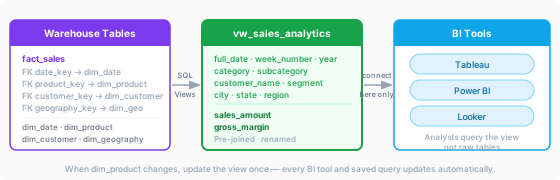
The query layer is the interface between your warehouse tables and your users. Without it, analysts query raw fact and dimension tables directly — 15-line JOIN statements every time anyone wants a revenue number. When the schema changes, every saved analyst query breaks.
The query layer typically has two parts:
- Presentation layer (SQL views): Views that pre-join fact and dimension tables, rename columns to business-friendly names, and calculate common metrics. BI tools connect to these views, not raw tables.
- Data mart layer (optional): Subject-area schemas scoped to one team — a marketing mart, a finance mart. Built on top of the core star schema; no data duplication.
SQL — Query Layer Views for ClothCo
-- Presentation view: pre-joins the star schema for BI tool consumption
-- Analysts and BI tools connect to this view, not to raw fact/dimension tables
CREATE VIEW vw_sales_analytics AS
SELECT
    dd.full_date,
    dd.week_number,
    dd.month_name,
    dd.year,
    dp.product_name,
    dp.category,
    dp.subcategory,
    dc.full_name         AS customer_name,
    dc.segment           AS customer_segment,
    dg.city,
    dg.state,
    dg.region,
    dg.country,
    fs.quantity,
    fs.unit_price,
    fs.discount_amount,
    fs.sales_amount,
    fs.gross_margin
FROM fact_sales      fs
JOIN dim_date        dd ON fs.date_key      = dd.date_key
JOIN dim_product     dp ON fs.product_key   = dp.product_key
JOIN dim_customer    dc ON fs.customer_key  = dc.customer_key
JOIN dim_geography   dg ON fs.geography_key = dg.geography_key;
With the view in place, the original business requirement — revenue by product category per week — becomes a clean 10-line query:
-- BI query: revenue by product category per month
-- Runs against the view, not the raw star schema
SELECT
    year,
    month_name,
    category,
    SUM(sales_amount)   AS total_revenue,
    SUM(gross_margin)   AS total_margin,
    COUNT(*)            AS order_lines
FROM vw_sales_analytics
GROUP BY year, month_name, category
ORDER BY year DESC, month_name, total_revenue DESC;
Connecting BI Tools to the Query Layer
| BI Tool | Connection Method | Best for |
|---|---|---|
| Tableau | Live connection or extract | Visual analytics; ad hoc exploration by analysts |
| Power BI | DirectQuery or Import mode | Microsoft ecosystem; broad user base |
| Looker | LookML semantic layer on top of views | Enterprise self-service; governed metrics across multiple teams |
| Metabase | Direct SQL connection | Lightweight, open-source; quick to set up for smaller teams |
| dbt + BI | dbt Semantic Layer (metric definitions) | Consistent KPI definitions shared across all connected tools |
The rule: expose the presentation view (vw_sales_analytics) to your BI tool, never the raw fact table. This concentrates JOIN complexity in one place and makes the warehouse resilient to schema changes. When dim_product gains a new column, add it to the view — analysts see it automatically in every tool. For the KPI tracking patterns analysts apply once data is in a BI tool, the KPI examples guide covers the metrics warehouses are built to calculate.
Data Warehouse Best Practices
1. Never query staging tables from BI. Staging is for loading only. The data there is raw, untyped, and potentially duplicate. BI tools connect to the presentation layer exclusively. This boundary is not optional.
2. Use surrogate keys, not natural keys. Source system IDs can change, be reused, or collide across systems when two sources are combined. Surrogate keys are integers generated by the warehouse and independent of anything upstream. Build the habit from the first table.
3. Document the grain on the CREATE TABLE statement. Write it as a comment: -- Grain: one row per order line item. When a new engineer joins 18 months later, they should not have to guess. If two people on the team disagree about what a fact table row represents, the fact table is broken before a single row loads.
4. Build incrementally from day one. Full loads — truncate and reload — work for small tables but fail at scale. Design your ETL with incremental logic from the start: WHERE NOT EXISTS or WHERE loaded_at > last_run_timestamp. Retrofitting incremental logic onto a full-load ETL is painful and error-prone.
5. Run validation checks before go-live. At minimum: (a) row count in the fact table matches the source, (b) SUM(sales_amount) in the warehouse matches total revenue in the source, (c) no NULL values in any foreign key column. Catch data problems in testing, not in a VP's dashboard on Monday morning.
6. Version-control every SQL file. Every CREATE TABLE, INSERT, and CREATE VIEW statement belongs in a git repository. Use dbt for transformation SQL — it handles lineage, documentation, and automated testing. A warehouse whose SQL exists only on someone's laptop is a liability waiting to surface.
Common Mistakes That Kill Data Warehouse Projects
Mistake 1 — Starting with the tool. "We'll use Snowflake" is not a data warehouse strategy. Tool selection belongs after requirements, not before. Picking a cloud platform before defining business questions is building a house by choosing the brand of nails first. The tool is a consequence of requirements, not the starting point.
Mistake 2 — Trying to build everything at once. Your first deliverable should cover one subject area: sales orders, or marketing leads, or finance invoices — not all three. Ship the sales star schema in 4–6 weeks. That gives stakeholders something to react to and gives the team a schema pattern to repeat on the next subject area.
Mistake 3 — Using source system primary keys as fact table foreign keys. Source IDs can change, get reused, or collide across systems when two data sources are merged. An order ID from Shopify is not a stable foreign key in a warehouse that also ingests from your wholesale portal. Always generate surrogate keys in the warehouse.
Mistake 4 — Loading data without a staging layer. If a source system renames a column or changes a data type, your fact table INSERT breaks. A staging layer catches that upstream change before it reaches the presentation layer. Teams that skip staging spend hours debugging ETL failures caused by source changes they did not control and cannot roll back.
Mistake 5 — Applying SCD Type 1 everywhere because it is simpler. Type 1 (overwrite) destroys the ability to report history accurately. If your sales incentive structures changed midyear and customer segments shifted, you need Type 2 to attribute revenue correctly to the pre- and post-change periods. Know which dimensions change meaningfully over time and use Type 2 for those.
Mistake 6 — Skipping the query layer. Teams that connect BI tools directly to raw fact tables end up with hundreds of saved queries that duplicate JOIN logic. When dim_product changes, every query breaks. The query layer concentrates that logic in one place. It takes two hours to build and saves weeks of ongoing maintenance across the warehouse's lifetime.
FAQ — Building a Data Warehouse
How long does it take to build a data warehouse?
A minimum viable warehouse — one subject area, three to five dimensions, two working dashboards — takes 4–8 weeks with one to two dedicated engineers. The biggest time variable is source data quality. If your production database has nulls in key fields, duplicate records, and inconsistent date formats, ETL development expands significantly before a single row loads cleanly. A full enterprise warehouse covering multiple subject areas typically runs 6–18 months. Any estimate more precise than that range is a guess until a source data audit is complete.
What does it cost to build a data warehouse?
Cloud warehouse platforms charge per storage and compute: Snowflake starts around $23/TB/month for storage; BigQuery charges $0.020/GB for active storage and $5/TB for queries (or flat-rate slots for predictable costs). For a 1 TB warehouse with moderate query load, platform costs typically run $200–$2,000/month depending on query volume and compression. Add engineering time — a data engineer at $100K/year for six months is $50K — plus ETL tooling ($0–$500/month for open-source or managed) and BI tooling ($50–$150/user/month for Tableau or Power BI). Total first-year cost range for a small warehouse: $80,000–$300,000. The DW ROI Calculator helps map costs against time savings and analytical output for a business case.
Should I use Kimball or Inmon methodology?
Use Kimball for a first warehouse, a small-to-medium team, or any situation where "ship something in six weeks" matters. Kimball is bottom-up: start with the sales order business process, build its star schema, deliver it to stakeholders, then add the next business process. Inmon is top-down: design the full normalized enterprise data model first, then derive subject-area data marts from it. Inmon is appropriate for large enterprises with dedicated data architecture teams and an 18-month build runway. For a team of two or three building their first warehouse, Kimball ships and Inmon doesn't.
What is the difference between a data warehouse and a data lake?
A data warehouse stores structured, cleaned, modeled data optimized for SQL queries and business reports. A data lake stores raw, unstructured, or semi-structured data — JSON event logs, images, clickstream data — at low cost per GB. Data lakes are cheap to store things in and expensive to analyze from without prior transformation. The modern approach is a lakehouse: raw data lands in cloud object storage (S3, Azure Blob, GCS), structured in a warehouse format using Apache Iceberg or Delta Lake, then queried with the same SQL tools as a traditional warehouse. For a team deciding between the two patterns, the lakehouse question is primarily one of data team maturity and the volume of unstructured data the business actually uses.
What is SCD Type 2 and when do I need it?
SCD Type 2 (Slowly Changing Dimension Type 2) preserves history when a dimension attribute changes, by adding a new row rather than overwriting the old one. Each row gets valid_from and valid_to dates plus an is_current flag marking the active version. Use it when historical accuracy matters — if a customer moved from Standard to VIP in June and you need to attribute pre-June sales to Standard and post-June sales to VIP, Type 2 is required. If the change was a data correction (the wrong segment was entered originally), Type 1 (overwrite) is correct. The question to ask for every dimension: "If this attribute changes, do historical reports need to reflect the value at the time of the event, or only the current value?"
What is the query layer in a data warehouse?
The query layer is the abstraction between raw warehouse tables and business users or BI tools. It consists of SQL views or materialized views that pre-join fact and dimension tables, calculate common metrics, and expose column names in business terms — customer_key becomes customer_name, date_key becomes full_date. BI tools and analysts query the views, not the raw tables. When the underlying schema changes, you update the view once instead of fixing every saved query in every dashboard. The query layer is two hours of work that removes weeks of ongoing maintenance over the warehouse's lifetime.
What ETL tool should I use?
For most teams: Fivetran or Airbyte for extraction (they handle 150–300+ source connectors with no custom code), dbt for transformation (SQL-based, version-controlled, fully testable with dbt test), and dbt Cloud's built-in scheduler to start. This ELT stack requires no custom ETL code, runs entirely in SQL, and handles the full lineage from source to presentation layer out of the box. When pipeline complexity grows — dozens of sources, complex dependencies between pipelines, custom operators needed — graduate to Apache Airflow. The exploratory data methods that help you understand source data quality before you start building are covered in the exploratory data analysis guide.
What is a star schema in a data warehouse?
A star schema is a database design where a central fact table containing numeric measures sits at the center, surrounded by dimension tables containing descriptive attributes. The fact table connects to each dimension through a foreign key — a surrogate integer pointing to that dimension's primary key. When drawn on paper, the structure looks like a star: fact in the middle, dimensions radiating outward. Queries are fast because analysts only join the fact to the specific dimensions they need, and dimension tables are denormalized so there are no additional join hops to sub-tables. It is the standard schema for Kimball-style data warehouse design.
- Kimball, R., & Ross, M. (2013). The Data Warehouse Toolkit: The Definitive Guide to Dimensional Modeling, 3rd Edition. Wiley. The foundational reference for star schema design and dimensional modeling methodology.
- Inmon, W. H. (2005). Building the Data Warehouse, 4th Edition. Wiley. The original top-down enterprise data warehouse methodology and reference architecture.
- dbt Labs. dbt Documentation: What is dbt? docs.getdbt.com. The ELT transformation framework referenced in Phase 3; covers modeling, testing, and lineage.
- Fivetran. ETL vs ELT: What is the Difference? fivetran.com. Covers the technical distinction and when each pattern applies in modern cloud warehouse architectures.
- Kimball Group. Slowly Changing Dimensions Are Not Always as Easy as 1, 2, 3. kimballgroup.com. Detailed treatment of SCD Types 1, 2, and 3 with practical implementation guidance.