
You ran a regression in Excel's Data Analysis ToolPak and a summary output table appeared in a new sheet. Three separate blocks of numbers, dozens of values, and no legend. This guide walks through every row of that output — from Multiple R down to the Upper 95% column — using a consistent six-month dataset of advertising spend and revenue so you can follow the same logic in your own numbers.
The dataset runs from January to June: ad spend in thousands of pounds (£10k, £15k, £20k, £25k, £30k, £35k) against revenue in thousands of pounds (£85k, £110k, £132k, £158k, £171k, £194k). The output you get from running a simple linear regression on this data is used throughout every section below. If you haven't run the model yet, the step-by-step walkthrough in the linear regression guide shows you how to get there, or you can skip directly to our free linear regression calculator which generates the same output automatically.
The Three Sections of a Regression Output Table
Excel's output splits into three distinct blocks, each answering a different question.
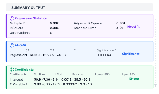
Section 1 — Regression Statistics tells you how well the model fits the data. How much of the variation in your outcome variable does the model account for?
Section 2 — ANOVA (Analysis of Variance) tests whether the model as a whole is statistically significant. Is there any evidence at all that your predictor variables are useful?
Section 3 — Coefficients gives you the equation of the line and tests each individual predictor variable. How steep is the slope, and can you trust that estimate?
Read them in that order and the whole output starts to make sense. Skip to the coefficients first and you'll often make errors — particularly around the p-value confusion covered in Section 2.
Section 1 — Regression Statistics (Model Fit)
The top block has five rows. Here's what each one tells you.
Multiple R
Multiple R is the correlation coefficient between the observed outcome values and the values your model predicted. For simple linear regression with one predictor, it's just the Pearson correlation between X and Y — which you can read more about in the correlation coefficient guide.
In this dataset, Multiple R = 0.992. That's a very strong positive correlation: months with higher ad spend consistently produced higher revenue. The value always sits between −1 and 1; negative values appear when the predictor and outcome move in opposite directions.
R Square (R²)
R² is Multiple R squared. Here, 0.992² = 0.985. This is the number most people want: it means the model accounts for 98.5% of the variation in monthly revenue. The remaining 1.5% comes from factors the model doesn't include — seasonality, promotions, competitor activity, random month-to-month noise.
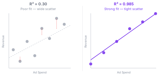
R² = 0.985 is unusually high for real business data. Most regression models in practice land somewhere between 0.3 and 0.7. A value near 1 isn't automatically good — it can signal overfitting, especially if your dataset is small (like these 6 months) or if you've included many predictors.
Adjusted R Square
Adjusted R² penalises you for adding more predictors to the model. Every new variable you add will increase R² a little even if it has no real predictive power. Adjusted R² corrects for that by factoring in the number of observations and predictors.
Here, Adjusted R² = 0.981. It's slightly lower than 0.985 because we have only six observations and one predictor — a small dataset where the correction is noticeable.
Which to use: R² or Adjusted R²?
For simple regression with one predictor, R² is fine to report. For multiple regression — or when you're comparing models with different numbers of predictors — use Adjusted R². It's the fairer comparison because it accounts for model complexity.
Standard Error
This is the standard deviation of the residuals — a measure of how far, on average, actual values stray from the model's predictions. With Standard Error = 4.97, you'd expect the model's predictions to be off by roughly ±£5k on a typical month.
Keep this number in mind. You'll see it again when calculating confidence intervals for predictions. It also gives you a quick sanity check on residuals: any observation with a residual larger than about 2× the standard error (here, more than roughly ±10) is worth examining for data errors or unusual circumstances.
One common confusion: this Standard Error (in the Regression Statistics block) is not the same as the Std Error column in the Coefficients block. They measure different things. The Regression Statistics SE describes overall prediction accuracy; the Coefficients SE describes the precision of a specific slope or intercept estimate.
Observations
Observations = 6. This is simply the number of data rows included in the model — January through June. With such a small sample, every statistical test in this output deserves skepticism. Regression with six data points can produce impressive-looking numbers that simply don't hold up once you add more data.
Section 2 — ANOVA Table (Overall Model Significance)
The ANOVA table tests a single question: does this model explain statistically more variation in Y than a flat line (the mean) would? The answer involves four values.
df (Degrees of Freedom)
Degrees of freedom for the Regression row equals the number of predictors — here, 1 (just ad spend). Degrees of freedom for Residual equals n − k − 1, where n is observations and k is predictors: 6 − 1 − 1 = 4. These values feed directly into the F and t calculations; you don't usually interpret them directly.
SS (Sum of Squares)
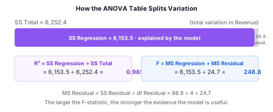
SS Regression (6,153.5) is the variation in revenue that the model explains. SS Residual (98.9) is the variation that remains unexplained. SS Total (6,252.4) is the total variation in monthly revenue around its mean (£141.7k). Their relationship is straightforward: SS Regression + SS Residual = SS Total, and R² = SS Regression ÷ SS Total = 6,153.5 ÷ 6,252.4 = 0.985.
MS (Mean Square)
MS is SS divided by its degrees of freedom. MS Regression = 6,153.5 ÷ 1 = 6,153.5. MS Residual = 98.9 ÷ 4 = 24.7. These two values are the ingredients for the F-statistic.
F and Significance F
The F-statistic (248.8) is MS Regression divided by MS Residual. A larger F means the variation your model explains is large relative to the unexplained noise. Significance F (0.000074) is the p-value for that F-statistic — the probability of seeing an F this large (or larger) if the true population slope were actually zero.
At 0.000074, Significance F is well below any conventional threshold (0.05, 0.01, or 0.001). The model is statistically significant.
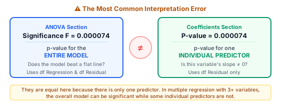
⚠ Significance F vs. individual p-values: these are not the same test
Significance F tests whether the whole model is useful. The P-values in Section 3 test whether each individual predictor's slope is different from zero. In simple regression with one predictor, they happen to give the same number. In multiple regression — with two, three, or more predictors — they can be very different. A model can have a highly significant overall F while some individual variables are non-significant, and vice versa. Never cross-reference these two to "double-check" your result.
Section 3 — Coefficients Table (Individual Effects)
This is the block that gives you the actual regression equation and tests each piece of it. For simple regression, there are two rows: Intercept and X Variable 1.
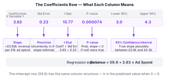
The Coefficients Column
The Intercept coefficient (59.9) is the predicted value of Y when X = 0 — the model predicts £59.9k revenue in a month with zero ad spend. This is often not meaningful on its own; it anchors the line mathematically but describes a scenario outside the data range.
The X Variable 1 coefficient (3.63) is the slope. For each additional £1k in ad spend, the model predicts an extra £3.63k in revenue. This is the core finding. The full equation reads: Revenue = 59.9 + 3.63 × Ad Spend. If you want to understand how that slope was calculated from the raw data, the linear regression guide walks through the least squares method in detail.
Standard Error (Coefficients Column)
The Std Error for X Variable 1 (0.23) is the standard deviation of the slope estimate — how much it would vary if you repeated the study many times with different samples from the same population. A smaller Std Error relative to the coefficient means a more precise estimate.
The ratio of coefficient to Std Error gives the t Stat: 3.63 ÷ 0.23 = 15.77. The intercept has its own Std Error (7.36) and t Stat (8.14), which test whether the intercept is different from zero.
t Stat
The t Stat tests whether a coefficient is statistically different from zero. With a t Stat of 15.77 for the slope, the estimate is 15.77 standard errors away from zero — extremely strong evidence that ad spend has a real effect on revenue. As a rough rule, a t Stat above about 2.0 (in absolute value) is statistically significant at the 5% level, though the exact threshold depends on degrees of freedom.
P-value
The P-value (0.000074) for X Variable 1 is the probability of observing a slope at least as extreme as 3.63 if the true population slope were actually zero. At 0.000074, this is overwhelmingly small — less than a 0.01% chance of getting this result by random noise if ad spend had no real effect. The intercept P-value (0.0012) tests whether the intercept is different from zero; it's also significant here, though the intercept's significance is rarely the main question.
Standard thresholds: p < 0.05 is usually called statistically significant, p < 0.01 strongly significant, and p < 0.001 very strongly significant. These are conventions, not laws — context determines what threshold is meaningful for your specific decision.
Lower 95% and Upper 95%
These form the 95% confidence interval for the slope: [3.0, 4.3]. This means the data are consistent with a true population slope somewhere between £3.0k and £4.3k revenue per £1k ad spend. It's a range of plausible values, not a probability statement about the specific value 3.63 — common wording like "95% chance the true slope is in this range" is technically incorrect.
The confidence interval is narrower when you have more data, more consistent measurements (lower Standard Error), and a more linear relationship. With six observations, [3.0, 4.3] is a reasonably tight interval — a consequence of the very high R².
Reading the Residuals Output
If you checked the "Residuals" box in the regression dialog before running, Excel adds a fourth table and optional plot below the main output.
The Residuals Table
Each row shows the fitted (predicted) value and the residual (actual minus predicted) for every observation:
| Month | Ad Spend (£000) | Actual Revenue (£000) | Predicted Revenue (£000) | Residual (£000) |
|---|---|---|---|---|
| January | 10 | 85 | 96.2 | −11.2 |
| February | 15 | 110 | 114.4 | −4.4 |
| March | 20 | 132 | 132.5 | −0.5 |
| April | 25 | 158 | 150.6 | +7.4 |
| May | 30 | 171 | 168.7 | +2.3 |
| June | 35 | 194 | 186.9 | +7.1 |
January's residual of −11.2 stands out. The model overpredicts January revenue by £11.2k — more than twice the Standard Error of 4.97. That's worth investigating. Perhaps ad spend in that month had a lag effect, or January had a seasonal dip that an advertising variable can't capture.
The Residual Plot
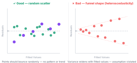
A healthy residual plot looks like random noise around y = 0 with no obvious pattern. What to watch for:
- Fan or funnel shape — variance increases (or decreases) with fitted values, violating the constant-variance assumption
- Curved pattern — the relationship between X and Y may not be linear; a quadratic term might fit better
- One or two extreme outliers — isolated points that the model fits badly, worth checking for data errors
With only six points, it's nearly impossible to diagnose these patterns reliably. The residual plot becomes much more useful with 30+ observations.
Statistical vs. Practical Significance
A result can be statistically significant without being practically meaningful — and vice versa.
Statistical significance (the P-value) tells you whether an effect is real, not zero. With enough data, even a slope of 0.001 can be statistically significant. It tells you the effect exists, not that it matters.
Practical significance is about whether the magnitude of the effect is large enough to care about in your specific context. A slope of 0.001 might be statistically significant in a dataset with 10,000 observations while being economically meaningless for every real decision you make.
In this dataset, the slope of 3.63 says each £1k of extra ad spend produces about £3.63k more revenue — a 3.63:1 return. That's both statistically significant (p = 0.000074) and practically interesting, since any marketing investment above a 1:1 revenue return is worth examining further.
The confidence interval [3.0, 4.3] adds further weight. Even the lower bound (3.0) represents a positive return. If the lower bound were negative, you'd need a different conversation about whether to continue the campaign at all.
| Statistical significance | Practical significance | What it means |
|---|---|---|
| ✓ Significant | ✓ Meaningful | Act on this — the effect is real and large enough to matter |
| ✓ Significant | ✗ Small effect | Real but trivial — large dataset detected a minor signal |
| ✗ Not significant | ✓ Large effect | May be real but data are too limited to confirm — collect more |
| ✗ Not significant | ✗ Small effect | No evidence of a meaningful effect |
What to Do With Your Regression Results
Once you've read the output, the next step depends on what you found.
If R² is low (below 0.3 in most business contexts), the model isn't capturing much variation. You might be missing important predictors, the relationship might not be linear, or the outcome variable might simply be too noisy to predict well from a single input. Try adding other variables or transforming X or Y (a log scale often helps when values span multiple orders of magnitude).
If Significance F is above 0.05, the model isn't statistically significant overall. With few predictors and small datasets, this often means you need more data before drawing conclusions.
If individual P-values are above 0.05 for some predictors but the overall F is significant, those variables may not be contributing much. Consider removing them one at a time and checking whether Adjusted R² improves.
If the model looks good — high R², low Significance F, significant slopes, and clean residual plots — you can use the equation for prediction and report your findings. Use the regression calculator to run what-if scenarios quickly without returning to Excel each time.
Before acting on any regression result, check whether the relationship is causal or merely correlational. The slope in this dataset shows a consistent association between ad spend and revenue, but it doesn't prove that spending more causes revenue to rise. Other confounding factors (seasonality, promotions, economic conditions) could explain part of the pattern. The correlation vs. causation guide goes deeper on this distinction.
How to Report Regression Results in Plain English
When writing up results for a business audience, translate the numbers directly:
Model fit: "The model accounted for 98.5% of the variation in monthly revenue (R² = 0.985, Adjusted R² = 0.981)."
Overall significance: "The overall regression was statistically significant (F(1,4) = 248.8, p < 0.001)."
Slope: "Each additional £1k of advertising spend was associated with an average £3.63k increase in revenue (b = 3.63, SE = 0.23, p < 0.001, 95% CI [3.0, 4.3])."
Equation: "The estimated regression equation is Revenue = 59.9 + 3.63 × Ad Spend."
Notice the phrasing "associated with" rather than "caused". Unless you have a randomised experiment, regression shows association, not causation. You should also note the sample size (n = 6) and that extrapolating beyond the observed range (£10k–£35k ad spend) may not be reliable.
For a formal report, include a table of the coefficients with standard errors, t statistics, p-values, and confidence intervals — the structure Excel already gives you. For a slide deck, the equation and R² are usually enough for the main finding, with the full table in an appendix.
Common Interpretation Mistakes
Confusing Significance F with coefficient P-values. As covered above, these test different things. This is the error most commonly found in tutorials that copy the Excel output without reading it carefully.
Treating R² as a percentage of data points. R² = 0.985 doesn't mean "98.5% of the data points lie on the line." It means the model explains 98.5% of the variance in Y. Some points can lie well off the line in a high-R² model if the variation is small everywhere.
Interpreting confidence intervals as probability ranges. The statement "there's a 95% probability the slope is between 3.0 and 4.3" is incorrect. The slope either is or isn't in that range; probability doesn't apply to a fixed value. The correct framing: "this interval was constructed using a method that captures the true slope 95% of the time in repeated sampling."
Assuming a low P-value confirms the model's assumptions. P-values and confidence intervals are only valid if the residuals are approximately normal, independent, and have constant variance. A statistically significant p-value doesn't mean those assumptions are met — that's what the residual plot checks.
Extrapolating beyond the data range. The equation Revenue = 59.9 + 3.63 × Ad Spend was fitted on data from £10k to £35k. Predicting revenue from £200k of ad spend — far outside that range — assumes the linear relationship continues indefinitely, which almost never holds in practice.
Misreading the two Standard Errors. The Standard Error in Regression Statistics (4.97) measures overall prediction accuracy. The Std Error in the Coefficients table (0.23) measures the precision of the slope estimate. These are different things with the same label.
Making Predictions from Your Regression Equation
The regression equation lets you plug in a new value of X and get a predicted Y. To predict revenue for a month with £28k ad spend: Revenue = 59.9 + 3.63 × 28 = 59.9 + 101.6 = £161.5k.
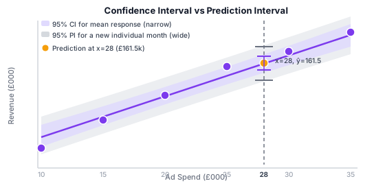
There are two distinct intervals for any prediction:
Confidence interval (CI) — a range for the average revenue across many months with this exact ad spend. At x = 28, the 95% CI runs from about £155k to £168k. This is a narrow band because it describes the mean response across repeated months, and averages are more stable than individual values.
Prediction interval (PI) — a range for one specific future month with £28k ad spend, accounting for all the random month-to-month variation on top of the model uncertainty. The 95% PI runs from about £147k to £177k — considerably wider than the CI. This is the interval to use when making a decision about a single upcoming month.
The linear regression calculator can generate both intervals for any X value you enter, so you don't need to work through the formula manually every time.
Interpreting Multiple Regression Output
When you add a second predictor (say, website sessions alongside ad spend), the output grows but the structure stays the same. The Regression Statistics and ANOVA sections look identical. The Coefficients table now has three rows: Intercept, X Variable 1, and X Variable 2.
Each slope in multiple regression is a partial slope: the expected change in Y per unit increase in that predictor, holding all other predictors constant. If the slope for ad spend changes from 3.63 to 2.80 when you add website sessions, that tells you the two predictors share some explanatory power — their effects overlap. The new slope of 2.80 is the ad spend effect after removing the variation that website sessions also explain.
Significance F and coefficient P-values can diverge substantially in multiple regression. The model overall may be significant (Significance F < 0.05) while one or more individual predictors have P-values above 0.05, meaning those particular variables don't add much once the other predictors are included. This is called multicollinearity when predictors are highly correlated, and it can make individual slopes hard to trust even when the overall model is good.
Adjusted R² becomes the right fit metric when comparing models with different numbers of predictors. A model with five predictors might have a higher R² than one with three, but a lower Adjusted R² — meaning the extra two variables didn't earn their place.
Quick Reference — Every Output Value at a Glance
| Value | Section | What it measures | Good sign |
|---|---|---|---|
| Multiple R | Regression Statistics | Correlation between observed and predicted Y | Close to 1 (or −1 for inverse) |
| R Square | Regression Statistics | Proportion of Y variance explained by model | Higher for the domain; near 1 is unusual |
| Adjusted R² | Regression Statistics | R² penalised for model complexity | Close to R²; use for model comparison |
| Standard Error | Regression Statistics | Typical prediction error (residual SD) | Small relative to the scale of Y |
| Observations | Regression Statistics | Number of data rows | At least 10–20 per predictor variable |
| df | ANOVA | Degrees of freedom for each SS component | Not interpreted directly |
| SS | ANOVA | Variance components (explained vs. unexplained) | SS Regression much larger than SS Residual |
| F | ANOVA | Ratio of explained to unexplained variance | Large (combined with low Significance F) |
| Significance F | ANOVA | p-value for the whole model | Below 0.05 |
| Coefficients | Coefficients | Slope (or intercept) in the regression equation | Direction and magnitude make sense |
| Std Error (Coeff.) | Coefficients | Precision of the coefficient estimate | Small relative to the coefficient |
| t Stat | Coefficients | Coefficient ÷ Std Error; how many SEs from zero | Absolute value above ~2 |
| P-value | Coefficients | Individual predictor significance | Below 0.05 (or your chosen threshold) |
| Lower/Upper 95% | Coefficients | 95% confidence interval for the coefficient | Interval excludes zero (consistent with significance) |
Frequently Asked Questions
What does Significance F mean in regression?
Significance F is the p-value for the overall regression model — the probability of getting an F-statistic this large or larger if none of your predictors actually had any effect on Y. A value below 0.05 is typically taken as evidence that at least one predictor in the model is useful. It answers the question "is this model better than just predicting the mean every time?"
What is a good R² value for regression?
That depends on the field. In physics or chemistry, R² of 0.99 is achievable. In economics or marketing, R² between 0.3 and 0.6 is often acceptable. In social sciences and health research, even 0.1–0.2 can be meaningful. The more important question is whether R² is good enough to make useful predictions in your specific context — an R² of 0.4 might be entirely adequate for strategic budgeting decisions.
How do I know if my regression slope is statistically significant?
Look at the P-value in the Coefficients section for that variable's row. If it's below 0.05, the slope is statistically significant at the 5% level — there's less than a 5% chance of seeing a slope this large if the true slope were zero. The t Stat also tells you: if its absolute value exceeds roughly 2, the slope is significant (the exact threshold depends on degrees of freedom).
Can I have a significant F but non-significant predictors?
Yes, this is quite common in multiple regression with correlated predictors. When two variables measure similar things, they compete to explain the same variation. Individually, neither one's slope clears the significance threshold — but together, they explain enough that the overall model is significant. This is a symptom of multicollinearity.
What does the intercept mean and do I need to interpret it?
The intercept is the predicted value of Y when all predictor variables equal zero. Often this is a hypothetical scenario outside the data range — in this dataset, revenue at zero ad spend (£59.9k). You'd interpret it only if zero is a realistic and meaningful value for all your predictors. For most business models, the intercept is just a mathematical anchor for the line.
Why do my Lower 95% and Upper 95% values not match what I'd expect?
The confidence interval width depends on the Standard Error of the coefficient, the t-critical value (which depends on degrees of freedom), and the sample size. With small samples, the t-critical value is large — which is why confidence intervals are wide with 10 observations and narrow with 1,000. Excel calculates this correctly; the interval may simply be wider than you expected because your dataset is small.
What does it mean if my R² is very high but my Significance F is poor?
This can happen with very small samples. With three observations and two predictors, R² will be 1.0 by definition — a line through two points is perfect — while Significance F may still be non-significant because there are no degrees of freedom left for residuals. High R² with non-significant F is usually a sign of an overfitted model on a tiny dataset.
Should I remove variables with high P-values?
Not automatically. Variable removal should follow a clear analytical rationale, not just a p-value threshold. If a variable was included based on domain knowledge (a known driver of the outcome), a non-significant P-value may mean the effect is too small to detect in your sample, not that the variable is irrelevant. That said, in predictive modeling — where the goal is accurate forecasts rather than understanding causes — removing non-significant predictors often improves generalisability.
What's the difference between the two Standard Error values in Excel's output?
Regression Statistics Standard Error (here, 4.97) is the residual standard deviation — the typical gap between actual Y and predicted Y across all observations. The Std Error column in the Coefficients section (e.g., 0.23 for the slope) is the standard deviation of the coefficient estimate, reflecting how precisely the slope is determined from the data. Same name, completely different things.
How many observations do I need for regression to be reliable?
A common rule of thumb is at least 10–20 observations per predictor variable. With six observations and one predictor, this analysis sits well below that threshold. The model gives an interesting signal, but all the statistics should be treated cautiously until more months of data are available. At six data points, any impressive-looking R² or p-value could be a sample-size artefact.
My residuals show a curved pattern — what does that mean?
A curved pattern in a residual plot usually means the relationship between X and Y isn't linear. The model predicts too high at the extremes and too low in the middle (or vice versa). The most common fixes are adding a quadratic term (X²) to the model, or transforming one or both variables using a log scale. If the curvature is mild, the linear model may still be useful for practical decisions within the data range.
Can I use this output to make predictions outside my data range?
Technically yes, but with significant caution. The linear relationship fitted between £10k and £35k ad spend may not continue at £50k or £100k — there are likely diminishing returns, budget constraints, or market saturation effects that the model can't see. Predictions within the original data range are on firmer ground. Predictions far beyond it are extrapolations that rest on the assumption that the same linear trend continues, which you can't verify from the data you have.
Conclusion
The three sections of a regression output each serve a distinct purpose: Regression Statistics shows how well the model fits, ANOVA tests whether it's statistically significant overall, and the Coefficients table gives you the equation and tests each individual predictor. Reading them in that sequence — fit first, then overall significance, then individual effects — avoids the most common interpretation errors.
The two values to watch most carefully: Adjusted R² (not raw R² when comparing models) and the Significance F vs. coefficient P-values distinction. Both pairs look similar in simple regression but behave very differently in multiple regression, where most real analyses live.
If you want to run the analysis on your own data without needing Excel's ToolPak, the linear regression calculator generates the same output with one-click predictions and confidence intervals. For a deeper look at how the slope and intercept are calculated in the first place, the linear regression guide covers the least squares method from scratch.
- Freedman, D., Pisani, R., & Purves, R. (2007). Statistics (4th ed.). W. W. Norton. Standard reference for regression inference and residual diagnostics.
- Wikipedia — Ordinary least squares. Covers the matrix derivation of the least-squares solution and the statistical properties of OLS estimators.
- NIST/SEMATECH e-Handbook of Statistical Methods. Section 4.4 — Confidence and prediction intervals for regression.
- Cook, R. D., & Weisberg, S. (1983). Diagnostics for heteroscedasticity in regression. Biometrika, 70(1), 1–10. The standard reference for residual plot diagnostics.
- Microsoft Support. Use the Analysis ToolPak to perform complex data analysis. Describes how to enable and use the Data Analysis ToolPak in Excel.