
A correlation coefficient summarizes the direction and strength of a specified type of association between paired variables. Pearson’s r measures linear association. Spearman’s rho measures monotonic association through ranks. Both range from −1 to +1 when defined; neither establishes causation.
This guide belongs to our Statistics category. Start with the sign and magnitude, then work through a five-pair calculation.
Read the number alongside the plot. The sign gives direction; the distance from zero gives strength for the type of association measured. A negative value can describe a strong relationship. Pearson’s r can be zero even when a clear curve connects the variables.
How to interpret a correlation coefficient
A positive coefficient means larger X values tend to occur with larger Y values. A negative coefficient means larger X values tend to occur with smaller Y values. “Tend to” matters: individual observations need not follow the overall pattern.
Read strength using the absolute value. A Pearson correlation of −0.9 represents stronger linear association than +0.4. The minus sign describes the direction, so it does not make the relationship weak or unimportant.
| Result | What it indicates | What it does not establish |
|---|---|---|
| Close to +1 | Strong positive linear association | That X causes Y |
| Close to −1 | Strong negative linear association | That the relationship is unimportant |
| Close to 0 | Little linear association | That no relationship exists |
| Exactly +1 or −1 | A perfect straight-line relationship in nonconstant observed data | Reliability beyond those observations |
There is no universal boundary separating a useful correlation from a useless one. Measurement reliability, the range sampled and the decision being made all affect interpretation. Report the actual value and explain its context rather than assigning a strength label alone.
Pearson correlation coefficient formula
Compare each value with its variable’s mean. When both values in a pair lie above their means, or both lie below, their deviations have a positive product. Opposite-sided deviations contribute a negative product.
r = Σ[(xᵢ − x̄)(yᵢ − ȳ)] ÷ √[Σ(xᵢ − x̄)² × Σ(yᵢ − ȳ)²]| Symbol | Meaning |
|---|---|
| xᵢ, yᵢ | The two values belonging to observation i |
| x̄, ȳ | Sample means of X and Y |
| Σ | Sum over all paired observations |
| r | Sample Pearson correlation coefficient |
The numerator measures whether deviations move together. The denominator scales this sum by variability in both variables. That scaling makes r unitless. The same relationship is r = sₓᵧ ÷ (sₓsᵧ), where sample covariance and both sample variances use the same n − 1 denominator. See our standard deviation explanation for the spread calculation.
If either variable is constant, its sum of squared deviations is zero. The denominator then vanishes and correlation is undefined. This is different from a defined coefficient equal to zero. The centered formula and constant-input behavior are documented in SciPy’s Pearson reference.
How to calculate correlation: a five-pair example
Use the hypothetical educational observations (1, 2), (2, 1), (3, 4), (4, 3) and (5, 5). These numbers represent paired measurements, not a measured study. Each column totals 15, so both sample means equal 15 ÷ 5 = 3.
Subtract 3 from each value, multiply the deviations within each row and square each deviation separately. Keep every X value matched with its original Y value.
| X | Y | X − x̄ | Y − ȳ | Product | Squared X deviation | Squared Y deviation |
|---|---|---|---|---|---|---|
| 1 | 2 | −2 | −1 | 2 | 4 | 1 |
| 2 | 1 | −1 | −2 | 2 | 1 | 4 |
| 3 | 4 | 0 | 1 | 0 | 0 | 1 |
| 4 | 3 | 1 | 0 | 0 | 1 | 0 |
| 5 | 5 | 2 | 2 | 4 | 4 | 4 |
| Total | 8 | 10 | 10 | |||
r = 8 ÷ √(10 × 10) = 8 ÷ 10 = 0.8
The positive value describes a positive linear association in these five pairs. It does not tell us that X causes Y or that the pattern will hold in a population. A significance test requires assumptions beyond this arithmetic.
Four scatter plots, four interpretations
Each point below represents one exact pair from a hypothetical dataset. The axes use the original numbers. Compare the plotted shapes before comparing the coefficients; the plots have different axis ranges.
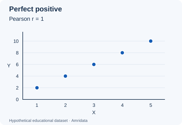


In the curved example, positive and negative contributions cancel. A straight-line summary misses the U shape. NIST’s scatter plot guidance describes plots as a way to inspect linear patterns, curves and unusual observations. Our guide to interpreting a scatter plot explains what to inspect.
Pearson versus Spearman correlation
A monotonic pattern moves consistently in one direction, although it may curve. Spearman correlation measures this association using ranks. It suits ordinal measurements and questions about ordering. It does not detect every nonlinear relationship: a U shape changes direction.
| Feature | Pearson’s r | Spearman’s rho |
|---|---|---|
| Input | Original numerical values | Ranks |
| Association | Linear | Monotonic |
| Perfect positive result | Increasing straight line | Perfectly agreeing rank order |
| Tied values | Used as observed | Usually assigned average ranks |
| Extreme observations | Can strongly affect the result | Often less sensitive to extreme magnitudes; influential observations still matter |
| Typical use | Numerical data with a relevant linear pattern | Ordinal data or a relevant monotonic pattern |
For hypothetical X = 1, 2, 3, 4, 5 and Y = 1, 4, 9, 16, 25, Pearson r ≈ 0.9811 while Spearman rho = 1. Every increase in X brings an increase in Y, so the ranks agree perfectly. The original points curve rather than following one straight line. Minitab’s comparison explains this distinction.

For ties, average the occupied ranks. Values 10, 20, 20, 40 receive ranks 1, 2.5, 2.5, 4. Spearman is Pearson correlation applied to these ranked values. The familiar shortcut involving squared rank differences assumes no tied ranks; average ranking handles the general case. See SciPy’s rankdata documentation.
Calculation, sample size and statistical inference
To calculate descriptive Pearson r, you need at least two paired numerical observations and nonzero variation in both variables. Normality is not required for the arithmetic. Keep the observational units aligned: January sales must match January advertising spend, not February spend by accident.
Population inference asks more. The conventional exact test of zero Pearson correlation assumes independent observations sampled from a bivariate normal population. Study design, model suitability and influential outliers need consideration. An automatic normality test is not a complete method-selection rule, and a large sample does not repair biased sampling or dependence.
Small samples can give unstable estimates. With just two nonconstant pairs, r must be +1 or −1 because two points define a line. Such a result supplies little evidence about a reliable population relationship.
A p-value describes how unusual a result at least as extreme would be under a specified null model. It is not the probability that the null hypothesis is true. Statistical significance depends on sample size and assumptions as well as the coefficient; practical importance depends on the question.
Report the number of complete pairs and, when inference is justified, a confidence interval using a suitable method. An interval communicates uncertainty that a rounded coefficient hides. SciPy documents Pearson testing and interval methods. No numerical p-value or interval is inferred from our teaching example.
Causation and the patterns a coefficient can miss
Imagine that hot days bring both higher ice-cream sales and more swimming. Temperature could explain an association between the two. This is an illustrative scenario, not a reported study. Confounding, reverse causation, selection effects, shared time trends and chance can all produce associations. Causal conclusions depend on study design and assumptions, not on crossing a correlation threshold. See correlation versus causation.
Inspect unusual points before reporting r. One distant observation can strengthen, weaken or reverse the coefficient. Check for recording errors and consider whether it belongs to the population of interest. Do not delete a valid observation merely because the coefficient improves without it.
A restricted range can change the apparent relationship. For example, studying only people of very similar heights gives a different view of height and weight than studying a broad height range. Combining groups can also hide within-group patterns or produce an association driven by differences between groups. Compare relevant subgroups when the study design supports that comparison.
Measurement error affects observed correlations. Independent random measurement error often reduces their magnitude, while other error structures can have different effects. Repeated measurements of one person and neighboring observations in a time series may be dependent, making standard uncertainty calculations unsuitable.
Missing values create another selection problem. Excluding incomplete pairs changes the analyzed sample. Remove or handle missingness at the pair level; deleting gaps separately in X and Y can match unrelated observations. Our missing-data guide covers the assumptions behind those decisions.
Correlation, regression and r²
Correlation summarizes association. Regression models an outcome in relation to predictors. R² describes model fit under a defined calculation. For ordinary least-squares simple linear regression with an intercept, fitted to the same paired data, R² = r².
Our worked example gives 0.8² = 0.64. The fitted line accounts for 64% of the observed variation in Y around its sample mean. This does not mean X causes 64% of Y. Squaring removes the direction: −0.8 also has a square of 0.64.
The identity does not extend automatically to models without an intercept, every regression method or Spearman’s rho squared. SciPy’s linear regression reference documents the relationship for its least-squares fit.
What changing units does to r
Swapping X and Y leaves Pearson correlation unchanged. Adding a constant to either variable or multiplying it by a positive constant also leaves r unchanged. Converting centimeters to meters therefore preserves it. Multiplying one variable by a negative constant reverses the sign; multiplying by zero makes that variable constant and the coefficient undefined.
Common mistakes to avoid
- Check a scatter plot before describing zero Pearson correlation as “no relationship.”
- Read sign and magnitude separately; −0.9 is not weaker than +0.4.
- Keep X and Y paired when sorting, filtering or handling missing values.
- Explain strength in context rather than applying a universal cutoff.
- Keep r, r² and p-values distinct: association, squared association and evidence against a null model answer different questions.
- Do not infer causation from significance or switch to Spearman merely because a curve exists.
Frequently asked questions
What does a correlation coefficient measure?
It measures the direction and strength of a specified association between paired variables. Name the coefficient: Pearson concerns linear association; Spearman concerns monotonic rank association.
What is its range?
Defined Pearson and Spearman coefficients lie between −1 and +1, including the endpoints.
What does a correlation coefficient of 0.8 mean?
For Pearson r, it describes a positive linear association. Its usefulness depends on the sample, measurements and purpose; it does not establish causation.
Is −0.9 stronger than +0.4?
Yes, in terms of linear association measured by Pearson r. Its absolute value is larger, and its direction is negative.
Does zero correlation mean independence?
No. Independent variables have zero population Pearson correlation when finite, nonzero variances exist, but the reverse does not generally hold. A sample r of zero cannot establish independence either.
Can a coefficient exceed 1?
A valid Pearson or Spearman coefficient cannot. A displayed value outside the range calls for checking the formula, data handling or numerical rounding.
When should I choose Spearman?
When ordering is meaningful, such as ordinal data, or when monotonic association answers your question. Inspect the plot; Spearman does not summarize all curved patterns.
What happens if one variable is constant?
Correlation is undefined because that variable has no variation. Reporting zero would imply a different result.
What is the difference between r and r²?
r retains direction. Its square does not. In simple ordinary least-squares regression with an intercept, r² equals the model’s R² on the same paired data.
Does a statistically significant correlation prove causation?
No. A significant result under a valid test does not rule out confounding, reverse causation or other explanations for association.
Related Statistics guides
References
- SciPy: Pearson correlation, calculation and inference
- SciPy: Spearman rank-order correlation
- SciPy: ranking tied values
- Minitab: Pearson and Spearman comparison
- NIST/SEMATECH: scatter plots
- SciPy: simple linear least-squares regression