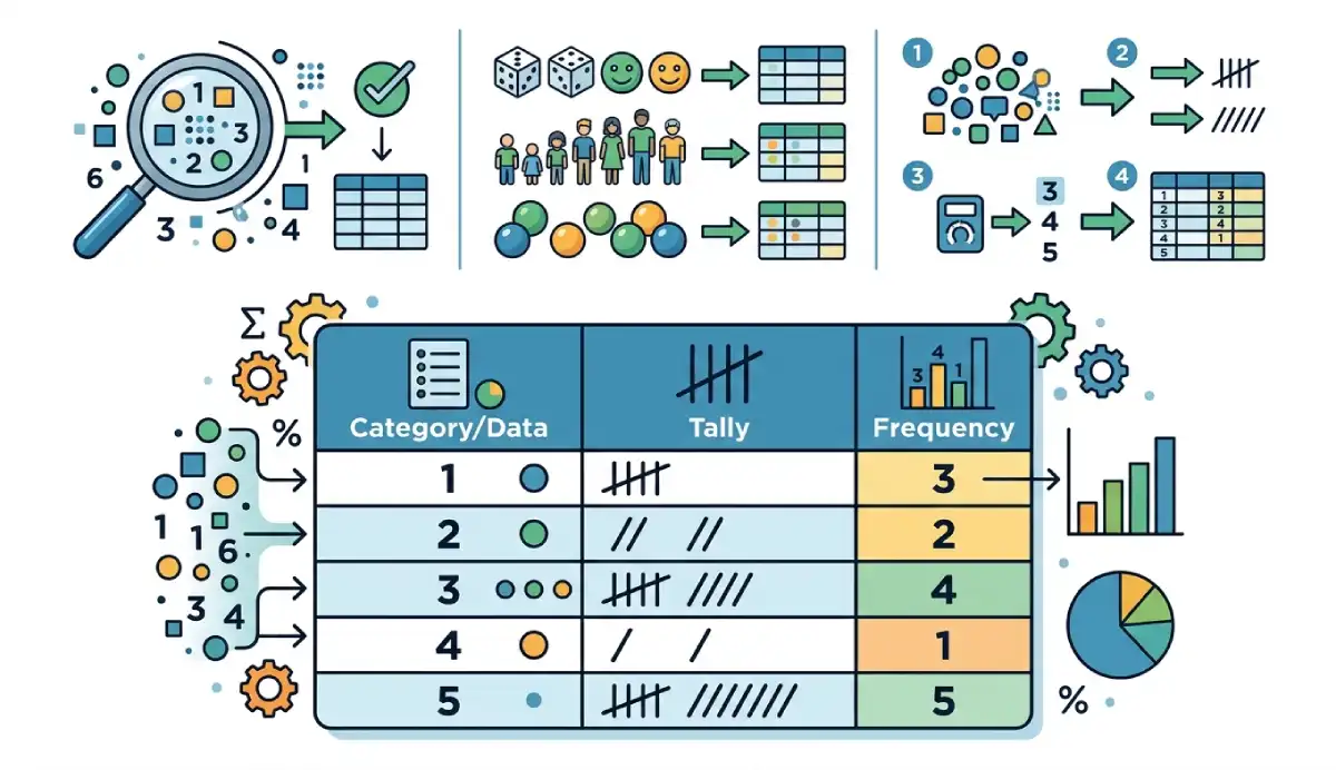
A frequency distribution table organizes data into values, categories, or intervals and shows how many observations belong to each group. Frequency means count. The frequencies add up to the number of included observations.
Numerical data can appear as exact values or as ranges. Extra columns can show each group’s proportion, percentage, or running total. This guide belongs to our Statistics category.
| Books read | Frequency |
|---|---|
| 0 | 1 |
| 1 | 2 |
| 2 | 2 |
| Total | 5 |
Here, two people read one book and two read two books. The total is five people, not five books. Start by checking what one observation represents.
What does a frequency distribution table contain?
A row identifies a value, category, or numerical class. Its other cells describe how often that group occurs. Tally marks are an optional counting aid, often bundled in fives; they are not needed in a finished table.
| Column | Meaning |
|---|---|
| Value or category | An exact outcome or label |
| Class interval | A numerical range |
| Frequency | Number of included observations in that row |
| Relative frequency | Frequency divided by the included total |
| Percentage frequency | Relative frequency multiplied by 100 |
| Cumulative frequency | Running total in a meaningful order |
| Class midpoint | Average of a finite class’s boundaries |
Relative frequency describes a share of the observed data [1]. A percentage is a percentage frequency, rather than a raw count. It does not automatically equal the probability in a wider population.
| Table type | Rows represent | Use when |
|---|---|---|
| Categorical | Labels or ordered categories | Responses are categories |
| Ungrouped numerical | Distinct numerical values | There are relatively few unique values |
| Grouped numerical | Numerical intervals | Many measurements need a shorter summary |
These choices concern the rows. Relative and cumulative columns are additions where appropriate: a grouped table can contain both. A numerical customer ID, however, is still an identifier; grouping IDs by magnitude rarely answers a useful question.
Ungrouped frequency distribution: books read
Suppose 20 students report how many books they read during one month. These are hypothetical observations, with no missing responses:
0, 1, 2, 1, 3, 2, 0, 4, 2, 1, 3, 2, 5, 1, 2, 3, 0, 4, 2, 1| Books read | Frequency | Relative frequency | Percentage | Cumulative frequency |
|---|---|---|---|---|
| 0 | 3 | 0.15 | 15% | 3 |
| 1 | 5 | 0.25 | 25% | 8 |
| 2 | 6 | 0.30 | 30% | 14 |
| 3 | 3 | 0.15 | 15% | 17 |
| 4 | 2 | 0.10 | 10% | 19 |
| 5 | 1 | 0.05 | 5% | 20 |
| Total | 20 | 1.00 | 100% | — |
The row for 2 books has six students. Its cumulative count is 14 because it includes everyone who read zero, one, or two books. The last cumulative entry already equals 20; adding the cumulative column would count students repeatedly.

How to make a frequency distribution table
- Define the variable. Here it is books read per student during one month. Include one response per student.
- Check the entries. Investigate blanks, impossible values, and inconsistent units. Zero books is a valid response.
- List distinct values in numerical order. Our rows are 0, 1, 2, 3, 4, and 5.
- Count each value. Mark each observation once. There are six occurrences of 2.
- Check the total. 3 + 5 + 6 + 3 + 2 + 1 = 20 students.
- Calculate shares. For 2 books, 6 ÷ 20 = 0.30, and 0.30 × 100 = 30%.
- Add running totals if useful. Through 2 books, 3 + 5 + 6 = 14. Thus 14 ÷ 20 = 70% read at most 2 books.
- Label the table. Name the variable, period, included sample, and any units or exclusions.
Use the Frequency Table Maker for your own data, then check its counts and interval labels against your intended rules.
Frequency, relative frequency, and cumulative frequency formulas
| Quantity | Formula |
|---|---|
| Total observations | n = Σfᵢ |
| Relative frequency | fᵢ ÷ n |
| Percentage frequency | 100fᵢ ÷ n |
| Cumulative frequency through row j | Fⱼ = f₁ + … + fⱼ |
| Cumulative relative frequency | Fⱼ ÷ n |
| Class width | Upper boundary − lower boundary |
| Class midpoint | (Lower boundary + upper boundary) ÷ 2 |
Here fᵢ is the frequency in row i, n is the included total, and Fⱼ is the running count through row j. Relative frequencies need n greater than zero. Weighted survey totals require a stated weighting method and should not be labeled ordinary observation counts.
Grouped frequency distribution: waiting times
Now consider 20 hypothetical waiting times, measured in minutes:
2, 4, 5, 7, 8, 10, 11, 12, 14, 15, 17, 18, 19, 20, 22, 24, 25, 27, 29, 30Use boundaries 0, 10, 20, and 30. Each ordinary interval includes its lower boundary and excludes its upper boundary. The final interval includes both boundaries, so the maximum is retained.
| Waiting time (minutes) | Frequency | Relative frequency | Percentage | Cumulative frequency | Midpoint (minutes) |
|---|---|---|---|---|---|
| 0 ≤ x < 10 | 5 | 0.25 | 25% | 5 | 5 |
| 10 ≤ x < 20 | 8 | 0.40 | 40% | 13 | 15 |
| 20 ≤ x ≤ 30 | 7 | 0.35 | 35% | 20 | 25 |
| Total | 20 | 1.00 | 100% | — | — |
The value 10 goes into the second interval, 20 into the third, and 30 remains in the final interval. Every observation enters exactly one class. The middle cumulative entry means 13 observations, or 65%, are below 20 minutes. “At most 20” would include the observation equal to 20 and give 14 instead.

Class limits, boundaries, width, and midpoint
For 10 ≤ x < 20, the boundaries are 10 and 20 minutes. The width is 20 − 10 = 10 minutes, and the midpoint is (10 + 20) ÷ 2 = 15 minutes. The midpoint labels a class center; it need not be an observed value.
A class labeled “10–19” can instead mean integer values 10 through 19. Those printed values are class limits. For measurements rounded to the nearest whole unit, boundaries of 9.5 and 19.5 may represent that class. The half-unit adjustment depends on measurement precision and rounding interpretation; it is not a universal instruction to add and subtract 0.5.
Do not combine “10–20” and “20–30” as inclusive classes without explaining where 20 belongs. Explicit inequalities remove this ambiguity. Boundary conventions can differ across references and software [2].
How to choose class intervals
Inspect the minimum and maximum, choose a manageable starting number of classes, and estimate width as the covered range divided by that number. Round to convenient boundaries, confirm that all observations fit, then inspect the resulting counts. Record the inclusion rule with the table.
Too few classes can conceal a cluster; too many can leave mostly empty rows. Our three waiting-time classes are a teaching choice, not an optimal bin count for every sample of 20. Try another reasonable width when the shape matters. Convenient rounding may change the number of classes. If every value is identical, one exact-value row may be more useful than inventing a range.
Frequency tables can contain text categories
| Preferred transport | Frequency | Percentage |
|---|---|---|
| Bus | 8 | 40% |
| Car | 6 | 30% |
| Bicycle | 4 | 20% |
| Walk | 2 | 10% |
| Total | 20 | 100% |
Bus is the most common response. Alphabetical order, survey order, or descending frequency may help readers find categories. These transport labels have no inherent ranking, so an ordinary cumulative distribution is not meaningful.
Ordered categories, such as low, medium, and high satisfaction, can support cumulative counts when the order is stated. A Pareto display instead accumulates shares after ranking categories by frequency; that is a different ordering.
Missing values change the percentage denominator
If 2 of 20 responses are missing, percentages may use all 20 records or only the 18 valid responses. If 9 valid responses are “Bus,” that is 45% of all records but 50% of valid responses. Label the denominator beside the table.
A separate “Missing” row can make exclusions visible. Do not remove blank responses and continue describing the denominator as 20 when calculations use 18. Keep zero unless the data definition explicitly marks it as missing. Our guide to handling missing data explains the broader choices.
Turn a frequency table into the right chart
| Data | Suitable display | What to check |
|---|---|---|
| Categories | Bar chart | Each bar represents a separate category |
| Distinct numerical values | Bar or dot display | Preserve numerical spacing |
| Numerical intervals | Histogram | Widths follow the interval boundaries |
| Ordered cumulative counts | Cumulative plot or ogive | Thresholds match the table convention |
Use a bar chart for the transport counts. For grouped measurements, the Histogram Maker provides a related display. A frequency polygon connects class-midpoint heights; it is another summary of grouped counts.
Unequal-width intervals need density heights
Equal-width histogram bars can use count heights. With unequal widths, use frequency density so each bar’s area represents its count. Relative-frequency density divides by the total as well, making the total area one [3].
| Interval | Frequency | Width | Frequency density |
|---|---|---|---|
| 0 ≤ x < 10 | 4 | 10 | 0.40 |
| 10 ≤ x < 20 | 3 | 10 | 0.30 |
| 20 ≤ x ≤ 40 | 1 | 20 | 0.05 |
Frequency density = frequency ÷ class width. The last bar is twice as wide, but its height is only 1 ÷ 20 = 0.05. Its area is 20 × 0.05 = 1 observation. Using count heights would exaggerate the area of the widest class. See the histogram guide for more on reading these displays.

How to read the table—and what grouping hides
In the books table, the mode is 2 books: it has the largest frequency, 6. Exactly 30% read 2 books, while 70% read at most 2. The mean, median, and mode guide explains how these summaries differ.
In the waiting-time table, 10 ≤ x < 20 is the highest-frequency class, containing 40% of observations. That does not reveal the exact raw-data mode. For unequal-width classes, distinguish the largest count from the highest density.
Grouping loses the exact positions within each interval. From the grouped table alone, you cannot recover the exact minimum, maximum, or number below 15 minutes. Moving an observation from 11 to 19 minutes would leave its class unchanged but alter that threshold count.
A midpoint-based mean is an estimate [4]: Σ(fᵢmᵢ) ÷ n, where mᵢ is the class midpoint. Our grouped estimate is (5 × 5 + 8 × 15 + 7 × 25) ÷ 20 = 16 minutes. The original waiting times average 15.95 minutes. Keep the raw data when exact results are needed.
Common mistakes to check before sharing
- Counts do not add to the included sample size.
- Intervals overlap, leave gaps, double-count a boundary, or omit the maximum.
- Numbers sort as text, putting 10 before 2.
- Percentages use an unstated or incorrect denominator.
- A cumulative count is read as an exact-value count, or cumulative rows are added together.
- Nominal categories receive an unexplained cumulative order.
- Midpoints are treated as original measurements.
- Unequal-width histogram bars use misleading count heights.
Independently rounded percentages may total 99.99% or 100.01%. For instance, three equal counts produce 33.33% each, totaling 99.99%. Calculate from full precision, disclose rounding, and do not silently adjust one category to force a displayed 100%.
Frequently asked questions
What is a frequency distribution table?
It lists values, categories, or intervals alongside the number of observations in each group.
How do you make a frequency distribution table?
Define the observations, check entries, choose rows, count each group, and verify the total. Add percentages or running totals when useful.
What is the difference between grouped and ungrouped tables?
An ungrouped numerical table keeps exact values as rows. A grouped table combines values into intervals and loses detail within them.
How do you calculate relative frequency?
Divide a row’s count by the included total. Six out of twenty is 0.30, or 30%.
What does cumulative frequency mean?
It is the running count through an ordered row. Through 2 books, our table includes 0, 1, and 2 books.
How do you choose class width?
Use the range and a manageable number of classes as a starting point, then check coverage and the resulting pattern. There is no universally best width.
Where does a value on a class boundary belong?
Follow the declared rule. Here 10 enters the second waiting-time class, 20 enters the third, and the final class includes 30.
Can a frequency table contain text?
Yes. Category labels such as Bus and Car can have counts and percentages, without an inherent cumulative order.
Why might percentages not total 100%?
Independent rounding can create a small discrepancy. A larger mismatch may indicate an omitted category or a wrong denominator.
Is a frequency table the same as a histogram?
No. The table records counts as numbers; a histogram displays numerical intervals as bars whose widths follow the intervals.
References
- OpenStax, Introductory Statistics 2e, §1.3: Frequency, Frequency Tables, and Levels of Measurement
- OpenStax, §2.2: Histograms, Frequency Polygons, and Time Series Graphs
- NIST/SEMATECH e-Handbook: Histogram
- OpenStax, §2.5: Measures of the Center of the Data