
Linear regression finds the straight line that fits your data points best, then gives you a formula to predict Y from X and measure exactly how the two move together. It answers concrete business questions: how much revenue does each pound of ad spend generate? How does price affect demand? One method, one equation, one R² — and all three are readable inside Excel.
This guide covers the concept, the formula, a hand-worked business example, and three ways to run regression in Excel — including how to interpret every row of the output table. It belongs to our Statistics category. If your data is ready now, skip ahead to our Linear Regression Calculator for instant slope, intercept, R², and p-value.
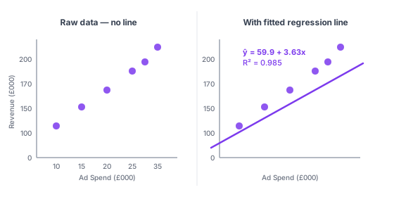
What is linear regression?
Linear regression is a statistical method that fits a straight line through a set of paired numeric observations. The line expresses how the dependent variable — the outcome you want to explain or predict — tends to change as the independent variable increases by one unit.
The term "regression" comes from Francis Galton's 1886 study of height inheritance. He found that the children of tall parents tended to be shorter than their parents — their heights "regressed" toward the population mean. The name stuck, and the method spread across statistics, economics, and business analytics over the century that followed.
Simple linear regression uses one X variable to predict one Y variable — the version this guide focuses on. Multiple linear regression extends the method to two or more X variables, adding one coefficient per predictor. The core mechanics are identical; the output table just gets more columns.
Linear regression is the right tool when you want to do one of two things. First, quantify the relationship: how much does Y change per unit of X, and how reliable is that estimate? Second, predict: given a new X value you haven't measured yet, what Y should you expect?
The When not to use section below covers the five situations where regression gives misleading results even when the R² looks respectable.
Real-world business applications
Linear regression works whenever you have paired numeric data and a reason to believe one variable drives the other. Here are four common use cases in business analytics.
| Use case | X (independent) | Y (dependent) |
|---|---|---|
| Forecast revenue from ad spend | Monthly ad budget (£) | Monthly revenue (£) |
| Predict demand from price | Unit selling price | Units sold per week |
| Estimate energy costs | Average outdoor temperature (°C) | Monthly energy bill (£) |
| Model salary by experience | Years in role | Annual salary (£) |
These four datasets are also the preset examples in our Linear Regression Calculator — load any of them to see the full output before entering your own numbers.
The key condition in every row: you have reason to believe X actually influences Y, not just that they happen to move together over your measurement window. Regression measures association. Business logic and domain knowledge determine whether the relationship is worth acting on. See the correlation vs. regression section below for where that distinction matters most.
The linear regression equation
Every simple linear regression produces one equation, written in two equivalent forms — the statistical notation and the slope-intercept form you may remember from school:
ŷ = b0 + b1x (statistical notation)
y = mx + c (slope-intercept form)

| Term | Name | What it tells you |
|---|---|---|
| ŷ | Predicted Y (y-hat) | The model's forecast for Y at a given value of X |
| b0 | Y-intercept | The predicted Y when X equals zero |
| b1 | Slope | How much Y changes for every one-unit increase in X |
| x | Independent variable | The input value you use to make the prediction |
Reading the slope takes one step: attach the units. If b1 = 3.63 and X is in £000, then each additional £1,000 of ad spend is associated with £3,630 more revenue on average. That single number — the slope — is usually the most commercially useful output from a regression.
The intercept needs context before you interpret it. For ad spend versus revenue, revenue at £0 spend has a reasonable meaning: repeat customers and organic demand. For something like years of experience versus salary, a salary at zero years falls outside the observed data range, and the intercept has no practical interpretation there. Don't over-read it in those cases.
Residuals
Actual observations rarely land exactly on the fitted line. The gap between the real Y and the predicted ŷ for each data point is a residual: residual = y − ŷ. If the model predicted £160,000 but actual revenue was £165,000, the residual is +£5,000.
Ordinary least squares regression finds the specific slope and intercept that minimise the sum of all squared residuals — meaning no other straight line produces a smaller total prediction error across the full dataset. That minimisation is what "fitting" the line means in practice.
How to calculate slope and intercept (step by step)
Here is the formula worked through with real numbers: six months of ad spend and revenue.
| Month | Ad Spend X (£000) | Revenue Y (£000) |
|---|---|---|
| Jan | 10 | 85 |
| Feb | 15 | 110 |
| Mar | 20 | 132 |
| Apr | 25 | 158 |
| May | 30 | 171 |
| Jun | 35 | 194 |
Step 1 — Calculate the means.
X̄ = (10 + 15 + 20 + 25 + 30 + 35) ÷ 6 = 22.5
Ȳ = (85 + 110 + 132 + 158 + 171 + 194) ÷ 6 = 141.67
Step 2 — Calculate the slope (b1).
b1 = Σ[(xi − X̄)(yi − Ȳ)] ÷ Σ[(xi − X̄)2]
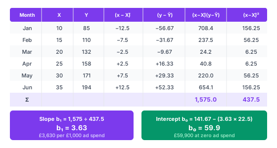
Σ[(xi − X̄)(yi − Ȳ)] = 1,575
Σ[(xi − X̄)2] = 437.5
b1 = 1,575 ÷ 437.5 = 3.63
Interpretation: each additional £1,000 of ad spend is associated with £3,630 more revenue on average.
Step 3 — Calculate the intercept (b0).
b0 = Ȳ − b1 × X̄ = 141.67 − (3.63 × 22.5) = 141.67 − 81.68 = 59.9
Interpretation: at £0 ad spend, the model predicts approximately £59,900 in baseline revenue — repeat purchases and organic traffic with no paid activity.
Step 4 — Write the equation.
ŷ = 59.9 + 3.63x, where x is monthly ad spend in £000 and ŷ is predicted revenue in £000.
Step 5 — Make a prediction.
If we plan to spend £28,000 next month:
ŷ = 59.9 + 3.63 × 28 = 59.9 + 101.64 = £161,540
You can verify every number in this example against the Linear Regression Calculator — load the ad spend preset and the results match exactly, including R², p-value, and the full output table.
Understanding R²: how well does the line fit?
R² (the coefficient of determination) answers one question: what proportion of the variation in Y does X explain? The result is a decimal from 0 to 1, usually reported as a percentage.

| R² range | What it means in practice |
|---|---|
| 0.90 – 1.00 | Very strong fit — X accounts for nearly all variation in Y. Common in physical measurements, rare in business data. |
| 0.70 – 0.89 | Strong fit — a good result for most business forecasting models with one predictor. |
| 0.50 – 0.69 | Moderate fit — X matters, but other factors explain a substantial share of Y's movement. |
| 0.30 – 0.49 | Weak fit — worth investigating, but don't base decisions on it without understanding what else drives Y. |
| < 0.30 | Poor fit — the line explains little. Consider adding more variables or switching to a non-linear approach. |
For the ad spend dataset, R² = 0.985 — 98.5% of the monthly revenue variation is explained by ad spend alone. That's unusually high for real business data; most single-variable forecasting models land between 0.50 and 0.80.
Two caveats to hold onto. A high R² does not prove causation — two completely unrelated variables that both trend upward over time can produce R² = 0.95 by coincidence. And in multiple regression, Adjusted R² is a more reliable metric than R² because regular R² always increases when you add variables even if they're useless. For simple regression with one X, the two are equal.
Related: in simple linear regression, R² equals r², where r is the Pearson correlation coefficient. See our correlation coefficient guide for the full connection between the two measures.
Statistical significance: is the relationship real?
A regression line always fits your data — that's what the algorithm guarantees. But is the slope meaningfully different from zero, or could it have appeared by chance in a small sample? The t-test for the slope answers this.
The null hypothesis is H0: b1 = 0, meaning X has no linear effect on Y. To test it, regression calculates a t-statistic:
t = b1 ÷ SE(b1)
SE(b1) is the standard error of the slope — how uncertain the estimate is given the sample size and the scatter around the line. A large t-statistic means the slope is large relative to its uncertainty. See our standard deviation guide for the underlying concept of dispersion that feeds into this calculation.
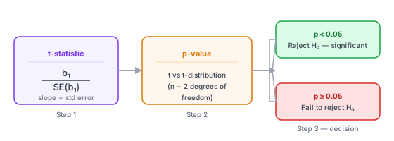
The p-value is the probability of observing a slope this large — or larger — if the null hypothesis were actually true. A p-value below 0.05 means you reject H0 and conclude the relationship is statistically significant at the standard threshold.
| p-value | Interpretation |
|---|---|
| < 0.001 | Very strong evidence of a real linear relationship between X and Y |
| 0.001 – 0.05 | Statistically significant at the standard threshold (p < 0.05) |
| 0.05 – 0.10 | Borderline — context dependent; don't treat as confirmed |
| > 0.10 | No significant evidence of a linear relationship at typical thresholds |
For the ad spend dataset with n = 6 observations, the t-statistic is 15.77 and p = 0.000074. The relationship is highly significant even with just six data points, because the scatter around the line is very small.
One common trap: statistical significance is not the same as practical significance. With a large enough dataset (n > 500), regression will flag almost any relationship as significant (p < 0.05) even when the slope is so small it's commercially worthless. Always report the slope size and its confidence interval alongside the p-value — not just whether the test passed.
Sample size note: With fewer than 20 observations, slope estimates are unstable and p-values can be unreliable in both directions. A relationship that tests as not significant with n = 8 might reach p < 0.05 with n = 30 on the same underlying data. Use our Linear Regression Calculator to check significance across different sample sizes before drawing conclusions.
How to run linear regression in Excel
Excel has three ways to get regression results. They trade speed for depth — the first takes 30 seconds and shows the equation; the third takes two minutes and returns the full statistical table including p-values and confidence intervals.
Method 1 — Scatter chart trendline (fastest)
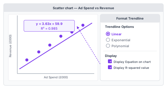
- Select your X and Y columns — both columns together, with headers included.
- Insert → Chart → Scatter. Choose Scatter with only Markers.
- Right-click any data point → Add Trendline.
- In the Format Trendline pane: select Linear; tick "Display Equation on chart"; tick "Display R-squared value on chart".
- Read the equation directly from the chart: y = 3.63x + 59.9, R² = 0.985.
What you get: slope, intercept, and R². What you don't get: p-values, standard errors, confidence intervals, or any diagnostic information. Use this method for a quick visual check or a chart that communicates the trend to an audience. Use Method 3 for any real analysis.
Method 2 — LINEST() function (embedded in sheet)
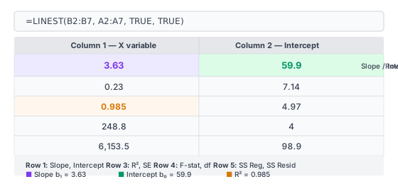
Formula: =LINEST(known_ys, known_xs, TRUE, TRUE)
- Select a blank 5×2 area (e.g., D1:E5).
- Type the formula:
=LINEST(B2:B7, A2:A7, TRUE, TRUE)— adjust ranges to match your data. - In Excel 365: press Enter. In older Excel: press Ctrl+Shift+Enter to confirm as an array formula.
- Read the results — Row 1 gives [b1, b0]. Row 3 gives [R², standard error of regression].
| Row | Column 1 (X variable) | Column 2 (Intercept) |
|---|---|---|
| 1 | Slope (b1) | Intercept (b0) |
| 2 | Standard error of slope | Standard error of intercept |
| 3 | R² (coefficient of determination) | Standard error of regression |
| 4 | F-statistic | Degrees of freedom (residual) |
| 5 | Regression sum of squares | Residual sum of squares |
To get the p-value from LINEST, calculate it separately: =F.DIST.RT(F_stat, 1, n-2), substituting the F-statistic from Row 4 and your sample size for n. For the ad spend example with n = 6: =F.DIST.RT(248.8, 1, 4) returns p = 0.000074.
Use LINEST when you need regression outputs embedded in a spreadsheet formula — for example, feeding the slope directly into another cell's calculation without building a separate summary table.
Method 3 — Data Analysis ToolPak (full output)
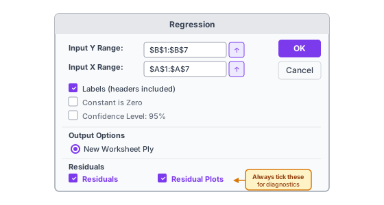
First-time setup: File → Options → Add-ins → Manage: Excel Add-ins → Go → tick Analysis ToolPak → OK. This is a one-time step.
- Data tab → Data Analysis → Regression → OK.
- Input Y Range: select your dependent variable column including its header (e.g., B1:B7).
- Input X Range: select your independent variable column including its header (e.g., A1:A7).
- Tick Labels — since you included headers in steps 2–3.
- Tick Residuals and Residual Plots — this generates the diagnostic chart you need to check model assumptions. It's the check most analysts skip, and skipping it is a mistake.
- Click OK. Excel generates the full output table on a new worksheet.
Reading the output table in full is covered in the Interpreting regression output section below. See also our Excel data analysis guide for the broader ToolPak workflow including descriptive statistics and histogram tools.
Prefer a web tool? Our Linear Regression Calculator returns the same full output — slope, intercept, R², p-value, confidence intervals, and a residual plot — just paste data from Excel or upload a CSV.
The four assumptions of linear regression
Regression always produces a line and statistics. These four assumptions determine whether you can trust those statistics. Mild violations are often acceptable for exploratory analysis. For formal inference — a forecast that drives a business decision — verify each one first.

L — Linearity
The relationship between X and Y should be approximately linear. Create a scatter plot before running regression — it takes ten seconds and can save you from an entirely wrong model. If the relationship curves (a U-shape, an S-shape, or any arc), regression forces a straight line through it and the results misrepresent the actual pattern. Fix: add a polynomial term (x²) or transform one variable (log Y is common for revenue and cost data).
I — Independence of observations
Each data point should be independent of the others. The most common violation is time-series data, where today's value depends on yesterday's — a problem called autocorrelation. Check the Durbin-Watson statistic in the ToolPak output. Values near 2 indicate no autocorrelation; values close to 0 or 4 signal a problem. If your data is monthly or quarterly over time, test for this before trusting the p-values.
N — Normality of residuals
The residuals (prediction errors) should be approximately normally distributed. This assumption applies to the residuals, not to the raw X or Y data — a distinction that some published guides get wrong. Your sales figures don't need to follow a bell curve; the gaps between predicted and actual values do. Check the residual histogram generated by the ToolPak's Residuals option, or the Q-Q plot in the calculator output.
E — Equal variance (homoscedasticity)
Residuals should have roughly constant variance across all values of X. If the residuals fan out as X increases — forming a funnel shape in the residual plot — the standard errors and confidence intervals are unreliable, even when the slope itself is accurate. The fix is either weighted least squares or a log transformation of Y. See our descriptive statistics guide for more on variance and how to measure it.
When not to use linear regression
Regression fits any dataset with a numeric X and Y. These five situations are where the method gives misleading results, however good the R² looks.
| Situation | Why regression fails here | Better approach |
|---|---|---|
| Non-linear relationship | Forcing a straight line through a curve understates the relationship at the extremes and overstates it in the middle | Polynomial regression, logarithmic transform, or a machine learning model |
| Binary or categorical Y | A yes/no outcome (churn or not, default or not) has no natural linear scale; predictions often fall outside 0–1 | Logistic regression |
| Very few data points (n < 15) | Slope and intercept estimates are unstable; a single outlier can dominate the entire result | Gather more data before modelling |
| Heavy outliers in X or Y | OLS minimises squared errors — large outliers are squared twice, pulling the line toward them disproportionately | Investigate outliers; consider robust regression |
| Extrapolating far beyond your data | The linear pattern you measured may not hold outside the observed X range | Limit predictions to X values within or near the observed range |
When in doubt, start with a scatter plot. If the relationship looks clearly non-linear, regression will produce a confident-looking but inaccurate result. See our scatter plot guide for how to read the patterns that signal a different model type is needed.
Correlation vs. regression: what's the difference?
Both methods measure relationships between numeric variables, and in simple linear regression r² = R². But they answer different questions and shouldn't be used interchangeably.
| Feature | Correlation (r) | Regression |
|---|---|---|
| Output | A single number from −1 to +1 | An equation: ŷ = b0 + b1x |
| Direction | Symmetric: r(X,Y) = r(Y,X) | Directional: X predicts Y, not the reverse |
| Main use | Measuring strength of association | Predicting Y, quantifying effect size |
| Implies causation? | No | No |
| Mathematical link | r is Pearson's correlation coefficient | b1 = r × (Sy ÷ Sx) |
Use correlation when you want to know how strongly two variables move together. Use regression when you want a predictive formula — specifically when you need to know how much Y changes per unit of X, or when you want to control for a third variable.
The mathematical link: in simple regression, the slope equals the correlation coefficient scaled by the ratio of standard deviations. That's why a correlation of r = 0 always gives a slope of zero, and r = 1 always gives a perfect fit. See our correlation coefficient guide and Pearson vs. Spearman comparison for the full picture.
Interpreting regression output: a complete guide
This is the section most tutorials skip. If a colleague or data team sends you a regression summary table, here is how to read every row — using the Excel ToolPak format and the ad spend dataset.

| Output label | Ad spend example value | What it means |
|---|---|---|
| Multiple R | 0.992 | Pearson correlation between X and Y — here, an extremely strong positive relationship |
| R Square | 0.985 | Ad spend explains 98.5% of the variation in monthly revenue |
| Adjusted R Square | 0.981 | Equals R² for simple regression; more important when you have multiple predictors |
| Standard Error | 4.97 | Average prediction error is ±£4,970 — the typical gap between predicted and actual revenue |
| Significance F | 0.000074 | p-value for the entire model — same as the slope p-value in simple regression |
| Intercept (Coefficient) | 59.9 | At £0 ad spend, predicted revenue is approximately £59,900 |
| X Variable 1 (Coefficient) | 3.63 | Each additional £1,000 of ad spend adds £3,630 predicted revenue |
| P-value (X Variable 1) | 0.000074 | Statistically significant — extremely unlikely to be a chance result |
| Lower 95% | 3.00 | The true slope is very likely at least £3,000 per £1,000 ad spend |
| Upper 95% | 4.26 | The true slope is very likely at most £4,260 per £1,000 ad spend |
The Coefficients section is where most of the actionable information lives. The slope's p-value tells you whether the relationship is statistically real; the 95% confidence interval tells you how precise the slope estimate is. A wide interval — Lower 95% far from Upper 95% — means the sample is too small to pin down the effect precisely, even if p < 0.05.
Making predictions: confidence intervals vs. prediction intervals
Once you have a regression equation, you can predict Y for new X values. But you need the right type of interval around that prediction, depending on what exactly you're forecasting.
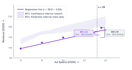
Confidence interval (CI) for the mean response: the range where the average Y is likely to fall for many observations at a given X value. Useful for scientific or population-level questions where you're estimating a true average.
Prediction interval (PI) for a new individual observation: the range where a single future Y value is likely to fall. This is wider than the CI because individual observations vary more than means do. For business decisions — forecasting next month's revenue at a specific ad spend — the PI is the interval to use.
For the ad spend dataset, predicting at x = £28,000:
- Point prediction: £161,540
- 95% Confidence Interval: approximately £155,000 – £168,000 (average revenue in months with £28,000 spend)
- 95% Prediction Interval: approximately £147,000 – £176,000 (range for next month specifically)
Prediction intervals widen as X moves away from the mean of your observed data (X̄ = £22,500 for this dataset). Predictions near the middle of your X range are most precise; predictions at the edges carry more uncertainty. The Linear Regression Calculator returns exact CI and PI values for any X you specify.
Common mistakes in linear regression
- Assuming correlation means causation. Two variables can rise together because both are driven by a third factor (the broader economy growing, say), or by complete coincidence over a short time window. High R² and low p-value only tell you the statistical relationship is real in your data — not that X causes Y. Business logic and controlled experiments are what establish causation.
- Skipping the residual plot. Most analysts stop at R² and p-value. The residual plot (residuals against fitted values) shows whether the model assumptions hold — linearity, constant variance, and the absence of outliers pulling the line off course. Run it every time. It takes 15 seconds in the ToolPak and can expose a badly misspecified model that looks fine on paper.
- Extrapolating beyond the observed range. Your model is calibrated for the X values you measured. Predicting revenue for an ad spend 10× higher than any month in your training data assumes the linear relationship continues indefinitely — an assumption with no support in the data you collected. Treat predictions outside the observed range with real caution.
- Too few data points. With n = 6, you can get a slope of 3.63 and R² = 0.985, as in this article's example. But the confidence interval is relatively wide (3.0 to 4.3), and a single unusual month would shift all the statistics noticeably. For stable inference, aim for at least 20–30 data points; for detecting small effects, you may need 100 or more.
- Confusing statistical significance with practical significance. With large datasets, even a slope of 0.001 can reach p < 0.001. That's statistically real but commercially irrelevant. Report the slope value and its confidence interval — not just the p-value — so the actual effect size is visible to whoever reads the analysis.
Frequently asked questions
What is linear regression in simple terms?
Linear regression finds the straight line that best fits a set of paired data points and gives you an equation for it. The equation tells you how much Y changes on average when X increases by one unit, and lets you predict Y for new X values you haven't measured.
What is the formula for linear regression?
The simple linear regression equation is ŷ = b0 + b1x, where ŷ is the predicted Y value, b0 is the y-intercept (predicted Y when X = 0), b1 is the slope (how much Y changes per unit X), and x is the value of the independent variable. Slope and intercept are calculated using ordinary least squares — the method that minimises the total squared prediction error across all data points.
What is the difference between simple and multiple linear regression?
Simple linear regression uses one independent variable (X) to predict Y. Multiple linear regression uses two or more (X1, X2, ..., Xn), giving the equation ŷ = b0 + b1x1 + b2x2 + ... Each coefficient in the multiple case represents the effect of that variable while holding the others constant. Use multiple regression when one X doesn't explain enough variation in Y, or when you need to control for a confounding variable.
What does R² mean in linear regression?
R² (the coefficient of determination) is the proportion of Y's variation that X explains, expressed as a decimal from 0 to 1. R² = 0.75 means 75% of the ups and downs in Y are captured by the fitted line; the other 25% reflect factors the model doesn't include. A good R² depends on context — 0.70 is strong for many business models; 0.30 may be acceptable in social science research where many factors influence outcomes.
What does the slope tell you in linear regression?
The slope (b1) is the average change in Y for every one-unit increase in X. If b1 = 3.63 and X is monthly ad spend in £000, then each additional £1,000 of ad spend is associated with £3,630 more revenue on average. A positive slope means X and Y move in the same direction; a negative slope means they move in opposite directions.
What are the assumptions of linear regression?
The four key assumptions — remembered as LINE — are: (L) the X-Y relationship is linear; (I) observations are independent of each other; (N) residuals (prediction errors) are approximately normally distributed — this applies to residuals, not to the raw data; (E) residuals have equal variance across all values of X (homoscedasticity). Check these using the residual plot generated by Excel's ToolPak or the calculator.
How do you run linear regression in Excel?
Three methods: (1) Add a linear trendline to a scatter chart and tick "Display Equation" — returns slope, intercept, and R² in 30 seconds. (2) Use =LINEST(known_ys, known_xs, TRUE, TRUE) as an array formula — returns a 5×2 output table including F-statistic. (3) Data Analysis ToolPak → Regression — returns the full output table including p-values, standard errors, confidence intervals, and residual plots. The ToolPak method is correct for any serious analysis. See the Excel section above for step-by-step instructions on all three.
How do you interpret regression results?
Focus on four numbers: slope (how much Y changes per unit X), R² (goodness of fit), the slope's p-value (is the relationship statistically real?), and the confidence interval for the slope (how precise is the estimate?). Then check the residual plot to verify the model assumptions hold. The full output table from Excel's ToolPak is explained row by row in the Interpreting output section above.
What is the difference between correlation and regression?
Correlation (r) measures how strongly two variables move together — a single number from −1 to +1. Regression gives a predictive equation that quantifies the effect of X on Y and lets you make predictions for new observations. Correlation is symmetric: r(X,Y) = r(Y,X). Regression is directional: X predicts Y, not the reverse. In simple linear regression, r² = R².
When should you not use linear regression?
When the relationship is non-linear (a scatter plot will show this clearly); when Y is a binary or categorical variable (use logistic regression instead); when you have very few data points (fewer than 15–20); when heavy outliers dominate the dataset; and when you're extrapolating predictions far beyond the range of your observed X values. The When not to use section above covers all five with specific alternatives for each.
What is ordinary least squares (OLS)?
Ordinary least squares is the estimation method used in standard linear regression. It finds the values of slope and intercept that minimise the sum of all squared residuals: Σ(yi − ŷi)². Squaring the residuals means large errors are penalised more heavily than small ones. The method has well-understood statistical properties that make p-values and confidence intervals straightforward to calculate and interpret. When people say "linear regression" without qualification, they almost always mean OLS regression.
How many data points do I need for linear regression?
A common guideline is 20–30 observations for simple linear regression to get stable estimates. With fewer than 15, slope and intercept estimates change substantially when you add a single data point, and confidence intervals are very wide. For detecting small effects (a correlation of r = 0.2, say), you may need 100 or more. For multiple regression, the guideline is roughly 10–20 observations per predictor variable. Use the Linear Regression Calculator to check significance and confidence interval width for your actual sample size before drawing conclusions.
How is linear regression different from logistic regression?
Linear regression predicts a continuous numeric outcome — revenue, temperature, salary. Logistic regression predicts a categorical outcome, almost always binary (yes/no, churn/retain, default/repay). The output of logistic regression is a probability between 0 and 1, not a continuous number. If your Y variable is a category or a probability rather than a measurement on a continuous scale, logistic regression is the right method.
Summary
Linear regression gives you three numbers that matter: a slope quantifying the effect of X on Y, an R² measuring how well the line fits, and a p-value confirming whether the relationship is statistically real. Excel's ToolPak delivers all three — plus standard errors, confidence intervals, and a residual plot — in about two minutes of setup.
The differentiating skill isn't running the analysis; it's reading the output correctly and knowing when the assumptions don't hold. Check the residual plot. Report the slope and confidence interval alongside the p-value. Don't extrapolate past the range of your data, and don't confuse a significant p-value with a commercially meaningful effect.
Use our Linear Regression Calculator to run the analysis on your own data — slope, intercept, R², p-value, confidence intervals, and residual plot, without needing to open Excel. For related methods, see our guide to descriptive statistics and data analysis methods.
- Galton, F. (1886). Regression towards mediocrity in hereditary stature. Journal of the Anthropological Institute of Great Britain and Ireland, 15, 246–263.
- Microsoft Support: LINEST function reference
- Microsoft Support: Use the Analysis ToolPak to perform complex data analysis