
A histogram is a graph that shows the distribution of numerical data by grouping observations into intervals called bins. The horizontal axis shows the intervals; the vertical axis shows counts, proportions, percentages, or density, depending on how the graph is scaled. A histogram makes it easier to see where values gather, how much they vary, and whether the distribution has gaps, tails, or more than one apparent peak.
Imagine 30 students taking a test. A list of 30 scores is precise, but not easy to scan. Group the scores into ranges such as 40–49, 50–59, and 60–69, then count the scores in each range. The resulting bars show which parts of the score scale contain the most students. That is the basic histogram meaning: values become bins, bins receive counts, and the counts describe a distribution.
Already have numbers to plot? Use AmriData’s Histogram Maker. This guide focuses on understanding the graph before you create one.
Part of AmriData’s Statistics guides. You can also browse the complete blog.
Histogram Definition: What Is a Histogram?
A histogram is a statistical graph for one quantitative variable. It divides the variable’s numerical scale into consecutive intervals and represents the amount of data in each interval with a rectangle. In an ordinary frequency histogram with equal-width bins, the height of each bar is the number of observations in that bin. In a density histogram, the bar’s area represents the share of observations.
The same graph may be called a histogram graph, a frequency histogram, or simply a histogram. Unlike a table of individual measurements, it deliberately groups nearby values. That grouping makes the overall pattern easier to see but hides some details. Two different lists of numbers can produce exactly the same bars.
- Best for: the distribution of test scores, heights, waiting times, prices, and other numerical observations.
- X-axis: an ordered number line divided into intervals (bins).
- Y-axis: frequency, relative frequency, percentage, or density; read the label.
- What to inspect: concentration, spread, skewness, apparent peaks, and gaps.
What Does a Histogram Show?
The histogram answers a question that a single average cannot: how are the observed values distributed? Two groups can have the same mean and very different patterns. One may be tightly clustered near its average; another may contain both low and high observations with little in the middle.
Start with the overall span of the data. Then identify the intervals with high counts, the sparsely populated regions, and whether the graph looks balanced on either side of its center. A long tail on the right suggests right skew; two separated high regions may suggest a mixture worth investigating. None of these impressions alone proves a population model or explains why the pattern exists.
A histogram does not show the exact value of every observation, the order in which values were collected, a time trend, or a cause-and-effect relationship. If you need the precise average or middle value, calculate it from the underlying numbers and see the mean, median, and mode guide.
Parts of a Histogram: Axes, Bars, and Bins
Reading the labels is more reliable than guessing from the shape. In a test-score histogram, the x-axis might be labeled “Score (points)” and the y-axis “Students (count).” A bar between 60 and 70 then tells you how many scores are at least 60 and below 70.
- X-axis: the observed variable, placed on a numerical scale; adjacent intervals have a meaningful order.
- Y-axis: the unit encoded by the graph’s height, such as count or percentage. For density, read area rather than height alone.
- Bin: a numerical interval that receives observations.
- Bar: the rectangle drawn over a bin, with height calculated from the chosen vertical scale.
- Bin width: the distance between a bin’s lower and upper boundaries, in the variable’s units.
- Bin boundaries: precise cutoffs that decide which interval receives a value.

Where Does a Score on the Boundary Go?
The intervals must not overlap. A clear rule is to include the lower boundary and exclude the upper boundary: [60, 70) includes 60 but not 70. The next bin, [70, 80), receives 70. In ordinary language, these mean “60 to under 70” and “70 to under 80.” A last bin may include the maximum endpoint when specified. Writing “60–70” and “70–80” without a convention leaves the placement of 70 ambiguous.
Histogram Example With Raw Data and Frequencies
Here is a complete, invented set of 18 test scores. It is small enough to count by hand: 52, 55, 57, 58, 61, 62, 63, 64, 66, 68, 70, 71, 72, 74, 77, 79, 82, 86.
Use four equal-width score intervals: 50 to under 60, 60 to under 70, 70 to under 80, and 80 to under 90. Count a score in exactly one interval.
Frequency table for the 18 scores
| Score interval | Scores in the interval | Frequency | Share of 18 |
|---|---|---|---|
| 50 to under 60 | 52, 55, 57, 58 | 4 | 22.2% |
| 60 to under 70 | 61, 62, 63, 64, 66, 68 | 6 | 33.3% |
| 70 to under 80 | 70, 71, 72, 74, 77, 79 | 6 | 33.3% |
| 80 to under 90 | 82, 86 | 2 | 11.1% |
| Total | 18 observations | 18 | 100% before rounding |
- OBSERVATIONS18One score per student
- MOST POPULATED BINS60–<80Six scores in each ten-point interval
- OBSERVED RANGE52–86Minimum and maximum score
The two middle bars together contain 12 of 18 scores, or 66.7% of the sample. The frequency is lower at both ends. It is reasonable to say the observed values are concentrated between 60 and under 80; it would be premature to call this small sample normally distributed. We also cannot recover the exact scores from the four rectangles alone.
These intervals were selected for clarity, not because every plotting program would choose them. An automatic histogram might begin at 52 rather than 50, or divide the range into a different number of bins. In that case its frequencies may differ while the underlying 18 values stay the same.
How to Read and Interpret a Histogram
Read the graph in a fixed order. First identify what was measured and in which units; a spread of 10 means something different for milliseconds and years. Next check the horizontal boundaries and the vertical scale. Only then describe the shape.
- Check the variable and sample. Are the observations student scores, individual transaction values, or something else? How many were collected?
- Read the bins. Note their boundaries, widths, and whether any intervals are empty.
- Read the vertical unit. “6 students” is not the same quantity as “33.3%” or a density of 0.0333 per point.
- Look for the center. Identify the numerical region where observations cluster, without pretending the bar chart gives an exact mean.
- Look for spread. Compare the occupied range and the width of the central group of bars.
- Inspect shape. Is it roughly balanced, asymmetric, flat, or marked by more than one apparent peak?
- Investigate the edges. Empty bins, long tails, or isolated low bars may deserve a look at the original data.
- Try different bins. Ask whether your impression survives reasonable changes in bin width and starting boundary.
Center and Spread Are Different Questions
The tallest interval is a modal bin under the current grouping; it is not necessarily the exact mode of the raw observations. To compare numerical centers, use the mean and median. To quantify variation, calculate range, interquartile range (IQR), or standard deviation as appropriate. A histogram supplements those summaries by showing what a single number leaves out.
What Do Gaps and Extreme Bars Mean?
An empty interval can reflect a genuine gap, the way a machine records measurements, or a sample that happens to contain no values there. A small bar far from the rest may suggest unusual observations. It does not prove an outlier, and it is not permission to delete data. Check the original records, units, and measurement process before acting.
Common Histogram Shapes
Shape names are shorthand for visible patterns, not diagnoses. A few observations or an unfortunate bin choice can create peaks and tails that disappear when you redraw the graph.

Symmetric and Bell-Shaped
A roughly symmetric histogram has a comparable overall pattern on either side of its central region. A bell-shaped histogram has higher bars near the middle and decreasing heights toward the tails. Many bell-shaped patterns are approximately symmetric, but a symmetric distribution need not be bell-shaped or normally distributed.
Right-Skewed (Positively Skewed)
Most observations are toward the lower part of the range, with a longer or thinner tail extending to larger values. Waiting times, order amounts, and incomes can show this pattern in some datasets, though not all. Define skew by its tail and asymmetry; the mean–median order is not a universal definition.
Left-Skewed (Negatively Skewed)
Observations cluster toward higher values while a tail extends toward lower ones. Imagine a relatively easy assessment on which most scores are high but a few students score far below the main group. That could produce a left-skewed histogram, but the data and binning decide.
Unimodal, Bimodal, and Multimodal
Unimodal describes one prominent peak; bimodal describes two apparent peaks; multimodal describes more than two. A bimodal graph may motivate checking whether measurements came from different groups or processes. It does not establish that exactly two populations were mixed. Changes to boundaries or sample size can produce or remove apparent peaks.
Uniform-Like
Bars of approximately similar height across the observed range suggest a relatively even distribution. They do not need to be identical. A flat-looking histogram from a small sample might simply be a result of random variation or broad bins.
Types of Histograms: Frequency, Percentage, and Density
Different histogram types organize the same observations with different vertical units or accumulation rules. The choice changes what a bar means. Labels should make that choice explicit.
Common histogram types and their vertical scales
| Type | Meaning of display | Useful when |
|---|---|---|
| Frequency | Bar height gives the number of observations in each equal-width bin. | You want actual counts in one sample. |
| Relative frequency | Bar height gives the bin count divided by the sample total, with equal-width bins. | You want proportions, such as 6/18. |
| Percentage | Relative frequency multiplied by 100. | Percent is easier for readers than decimals. |
| Density | Area of a bar gives its share of observations; height = relative frequency ÷ bin width. | You need a probability-scaled view, especially with unequal widths. |
| Cumulative | Counts or proportions accumulate as bin boundaries increase. | You want to see how many observations fall below successive cutoffs. |
Frequency vs Relative Frequency: Same Data, Different Scale
For the 60-to-under-70 interval, the frequency is 6. The relative frequency is 6 ÷ 18 = 1/3, approximately 0.333, or 33.3%. In a percentage histogram the corresponding value is 33.3%. With equal-width bins and unchanged boundaries, switching from counts to shares scales the bars but does not change their overall shape.

Density Histograms and Unequal Bin Widths
For a density histogram, use density = bin frequency ÷ (total observations × bin width). Multiplying that height by its bin width gives the proportion in the bin. This matters with unequal widths: a wide bin may contain more values partly because it spans more of the number line.
Combine the example’s 60-to-under-70 and 70-to-under-80 intervals into one 60-to-under-80 interval. The new frequency is 12, but the bin is 20 points wide. Its density is 12 ÷ (18 × 20) = 0.0333 per point. The narrower 50-to-under-60 bin has density 4 ÷ (18 × 10) = 0.0222 per point. With heights scaled this way, their bar areas correctly represent 66.7% and 22.2% of the sample.
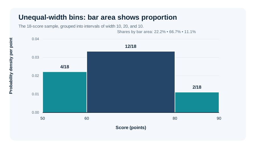
AmriData’s Histogram Maker currently offers frequency and relative-frequency views with equal-width bins; the density illustration here is a statistical explanation, not a claim that the tool has unequal-width density controls.
How Histogram Bins Work
Bins are the numerical intervals used to group raw observations. For the values 11, 13, 16, 18, 22, 24, 25, one reasonable set is 10 to under 15, 15 to under 20, 20 to under 25, and 25 to under 30. The resulting frequencies are 2, 2, 2, and 1. Another set of boundaries would place the same seven values into different groups.
Both bin width and starting position matter. A five-unit interval starting at 10 is different from one starting at 12. At a boundary, an observation may move from one rectangle to its neighbor; no observation itself has changed. When you compare two histograms, check whether they use compatible bins before comparing their heights.
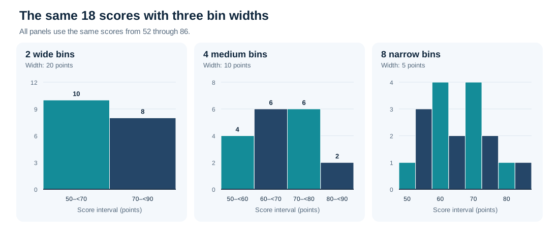
Why Bin Width Changes the Picture
Too few bins merge nearby details and can hide a gap or a second peak. Too many bins may make random fluctuations look like distinct features. The 18 test scores below appear as two broad bins, four moderate bins, and eight narrower bins. All three panels were calculated from exactly the same observations, and each counts 18 scores in total.
How Many Bins Should a Histogram Have?
There is no universally correct bin count. The best practical choice depends on the number of measurements, their range, any unusual observations, and what you are trying to learn. Automatic rules produce starting points, not final verdicts. Compare sensible alternatives and report the bin settings when small changes materially affect your conclusion.
Common starting rules for histogram bins
| Method | Formula | What it estimates |
|---|---|---|
| Sturges | k = ⌈1 + log₂(n)⌉ | Number of bins; simple for relatively modest samples. |
| Square-root | k ≈ √n | Number of bins; a quick rule of thumb. |
| Freedman–Diaconis | h = 2 × IQR × n−1/3 | Bin width based on middle-50% spread. |
| Scott | h = 3.5 × s × n−1/3 | Bin width based on standard deviation. |
Here n is the observation count, k is the number of bins, h is the bin width, IQR is the interquartile range, and s is sample standard deviation. A software implementation must still choose usable boundaries and handle exceptional cases, such as zero IQR or constant observations.
Sturges and the Square-Root Rule
With 100 observations, the square-root rule suggests roughly 10 bins. Sturges suggests ⌈1 + log₂(100)⌉ = 8 bins. Neither result means the histogram must use that count. Large or unusually shaped datasets can need a different approach.
Freedman–Diaconis and Scott’s Rules
Freedman–Diaconis uses the IQR, which is less affected by the magnitude of extreme values than standard deviation. Scott’s rule uses standard deviation and can work well for some reasonably smooth distributions. Both estimate width rather than specifying a fixed count. If the chosen width is unsuitable or cannot be calculated, use judgment, another rule, and a direct inspection of the data.
How to Make a Histogram Step by Step
- Collect one numerical variable. Use raw observations rather than totals by department or product category.
- Check the data. Verify units, missing entries, and unusually large or small values.
- Find the observed minimum and maximum. They help you choose a useful horizontal range.
- Choose intervals. Start with equal widths and state how boundary values are assigned.
- Count observations in each bin. Every valid observation should contribute to exactly one interval.
- Draw the graph. Put the ordered numerical bins along the x-axis and frequency or another clearly labeled scale on the y-axis; draw adjacent rectangles.
- Label the chart. Include the measured quantity, units, and what the vertical values mean.
- Inspect another bin choice. Check whether apparent peaks or gaps persist before making claims.
Create a Histogram With AmriData
For a faster practical check, paste the 18 sample scores into the free Histogram Maker. It can group the values automatically or let you select a custom bin count, switch the y-axis between frequency and relative frequency, display summary statistics, and download a PNG. The tool chooses equal-width boundaries for its own range, so they may not match the manually chosen intervals in our table. Treat that as a binning difference, not an error in the score list.
Histogram vs Bar Graph: What Is the Difference?
A histogram summarizes numerical observations grouped into intervals. A bar graph compares values associated with separate categories. Bars commonly touch in a histogram and have gaps in a bar graph, but spacing is not the deciding rule. The meaning of the horizontal axis is.
Histogram and bar graph comparison
| Feature | Histogram | Bar graph |
|---|---|---|
| Main question | How are numerical values distributed? | How do category values compare? |
| X-axis | Intervals on a number line | Named categories |
| Typical bar order | Fixed in numerical order | Often rearrangeable |
| Bar width | Represents a numerical interval | Usually a design choice |
| Example | Individual student scores by score range | Number of students choosing each fruit |
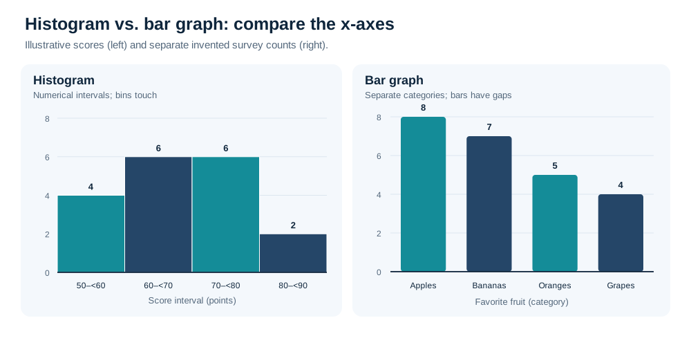
For a full comparison, read Histogram vs Bar Graph. If your variable is categorical, try the Bar Chart Maker rather than forcing categories into bins.
Histogram vs Box Plot
A histogram keeps the distribution visible across intervals and helps you notice peaks, tails, and gaps. A box plot compresses the observations into a median, lower and upper quartiles, an IQR, whiskers, and sometimes markers for potential outliers, depending on the plotting convention. It is often more compact when comparing several groups, but usually reveals less detail about peaks.
If your concern is whether a dataset has one or more clusters, a histogram is useful. If your concern is how group medians and IQRs compare, a Box Plot Maker may be clearer. These are complementary views, not competing definitions of the same graph.
Histogram vs Density Plot and Dot Plot
A histogram groups observations into hard-edged intervals. A density plot uses a smoothing method to produce a continuous-looking curve. The density plot has a bandwidth setting that can hide or exaggerate apparent peaks, just as a histogram depends on bins. Neither display uncovers an untuned “true” distribution. With only a handful of values, a dot or strip plot often communicates more because individual observations remain visible.
When Should You Use a Histogram?
Choose a histogram when the question concerns the distribution of numerical values. It is suitable for delivery times, measured heights, production errors, transaction amounts, temperature readings, and numeric test scores. It can also work for appropriately grouped discrete quantitative values; numerical data do not need to be perfectly continuous. If a variable takes only a few possible integer values, however, a dot plot may be easier to read.
Do not use a histogram to compare departments or brands, show change over time, or describe the relationship between two variables. A bar chart suits categories, a line graph suits many ordered time trends, and a scatter plot suits paired numerical measurements. For a broader decision, see how to choose the right chart type.
Can a Histogram Show Whether Data Are Normal?
It can suggest that observations look roughly unimodal, symmetric, and bell-shaped. It cannot establish that the population follows a normal distribution. A different sample or bin width may produce a different picture. When a statistical method relies on a distributional assumption, supplement the histogram with a Q–Q plot, relevant subject-matter context, and formal checks where appropriate; none should be treated as infallible on its own.
Common Histogram Mistakes
- Putting labels into bins. Departments, colors, and identification numbers used as labels belong in category displays.
- Using too few or too many bins. Check whether broad grouping hides detail or narrow grouping creates a jagged picture.
- Ignoring the bin origin. Moving the first boundary can change which observations group together.
- Leaving the y-axis unexplained. Count, percent, and density have different meanings.
- Comparing heights across unequal widths. For a density display, bar area carries the proportional meaning.
- Rearranging the bins. Their position on the number line is part of the information.
- Calling a shape proof. A bell shape does not prove normality, and a lonely bar does not establish an outlier.
- Hiding the sample size or units. Ten observations and ten thousand observations do not support the same confidence.
- Picking bins to support a preferred story. Try defensible alternatives and disclose important choices.
Other presentation errors, including misleading scales and ambiguous labels, are covered in common data visualization mistakes.
Frequently Asked Questions About Histograms
What is a histogram in simple terms?
A histogram is a graph that groups numerical observations into ranges and shows how many observations—or what share—fall in each range.
What does a histogram tell you?
It describes where values are concentrated, their spread, and possible patterns such as tails, peaks, or gaps. It does not establish the cause of those patterns.
What is a bin in a histogram?
A bin is a numerical interval. For example, 20 to under 30 can be one bin for a set of measured values.
What does the height of a histogram bar represent?
In a frequency histogram with equal-width bins, it is the count. In a relative-frequency or percentage histogram with equal-width bins, it is a share. In a density histogram, bar area represents the share.
Do histogram bars always touch?
Adjacent nonempty bins normally have touching rectangles because they share a numerical boundary. Empty intervals can show gaps, and styling alone does not define the chart type.
How many bins should I use?
There is no fixed correct number. Start with a reasonable automatic rule and compare several sensible choices, taking account of sample size and data spread.
What is the difference between a histogram and a bar graph?
A histogram uses numerical intervals to show a distribution. A bar graph compares values across categories, such as products or departments.
Can a histogram show discrete data?
Yes, it can summarize suitable numeric counts or scores grouped into intervals. For very few distinct integer values, a dot plot or frequency plot may make the individual values clearer.
Can you calculate the mean from a histogram?
You can approximate a mean from grouped bin midpoints and frequencies, but the exact mean generally requires the raw data or more detailed totals.
Does a bell-shaped histogram prove normality?
No. A bell-like picture is compatible with some normal-like data, but sample size and binning can affect its appearance. Use additional diagnostics when the assumption matters.
How do I make a histogram online?
Collect numeric observations, enter them into a Histogram Maker, choose a bin setting, generate the chart, and check its labels and distribution.
Key Takeaways
- A histogram shows how one numerical variable is distributed over ordered value intervals.
- Bin boundaries and widths affect the appearance of the graph even when the original data stay unchanged.
- Check whether the vertical axis shows counts, shares, percentages, or density; with unequal-width density bins, area conveys proportion.
- Peaks, tails, gaps, and bell shapes are starting points for interpretation, not proof of a statistical model.
- Use a bar graph for categories and a histogram for a numerical distribution.
To remember the histogram definition, focus on the number line: one interval, one count or share, one place in the distribution. Start with a clear scale, inspect more than one sensible bin setting, and use the raw values for calculations that require precision. For the larger workflow around inspecting a dataset, see exploratory data analysis steps.
Related Statistics Guides and Tools
- Histogram Maker — create and download a histogram from raw numerical values
- Bar Chart Maker — compare distinct categories
- Mean, Median, and Mode — calculate measures of center from data
- Standard Deviation Explained — measure numerical spread
- Histogram vs Bar Graph — a focused comparison of the two chart types
- How to Choose the Right Chart Type — alternatives for other questions
- Exploratory Data Analysis — put distribution checks in context
← Back to all Statistics articles
Statistical References
- NIST/SEMATECH e-Handbook of Statistical Methods — Histogram. Frequency bins and exploratory uses of histograms.
- Penn State STAT 200 — Describing Data. Introductory distinction between categorical summaries and quantitative distributions.