
A correlation matrix is a square table of correlation coefficients between pairs of variables. Each cell describes the direction and strength of the association measured by the chosen method. The rows and columns list the same variables; a heatmap displays their coefficients using color.
Standard Pearson and Spearman coefficients range from −1 to +1 when defined. Matching cells mirror each other when they use the same observations and method. Valid self-correlations equal 1, but constant variables or too few usable observations can leave entries undefined.
This guide belongs to our Data Visualization category. Start with this Pearson matrix, calculated from five hypothetical observations:
| Variable | X | Y | Z |
|---|---|---|---|
| X | 1.00 | 0.80 | −1.00 |
| Y | 0.80 | 1.00 | −0.80 |
| Z | −1.00 | −0.80 | 1.00 |
How to read a correlation matrix
- Find the first variable in the rows: X, for example.
- Find the second variable in the columns: Y.
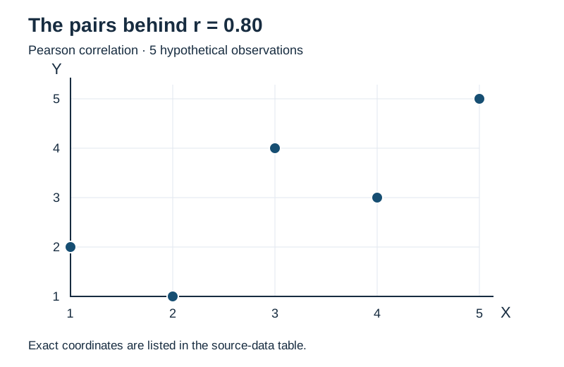
- Read their intersection. Here, X and Y have r = 0.80.
- Read the sign. Positive Pearson r describes an upward linear association; negative r describes a downward one.
- Read the magnitude in context. A value of −0.80 has the same absolute magnitude as +0.80. The negative sign does not make it weaker.
- Check the method and number of observations behind that cell.
- Inspect the paired data before drawing a conclusion.
In this example, X and Z have r = −1 because Z falls along an exact straight line as X increases. Y and Z have r = −0.80. These are descriptions of five invented observations, not evidence about a wider population.
There is no universal boundary between weak and strong correlation. Measurement quality, the field of study and the intended decision affect interpretation. Near-zero Pearson r can conceal a curved relationship. Use a scatter plot to inspect the relationship; NIST's guidance shows why shape and unusual points matter [1].
Why the matrix is square and symmetric
With p variables, the matrix has p rows and p columns. Correlating X with Y gives the same result as correlating Y with X on the same data. The diagonal compares each variable with itself, so defined entries equal 1. Do not fill an undefined diagonal with 1 just to complete the pattern.
Only p(p − 1) ÷ 2 off-diagonal pairs are distinct. Three variables give 3 unique pairs, five give 10 and ten give 45. A triangular display removes the mirrored duplicates. Every ordinary cell still concerns just two variables; it does not control for the remaining columns.
How to calculate a correlation matrix
Keep each observation on one row. The following hypothetical educational dataset produces the opening matrix. The exact negative relationship between X and Z is intentional for teaching.
| Observation | X | Y | Z |
|---|---|---|---|
| 1 | 1 | 2 | 5 |
| 2 | 2 | 1 | 4 |
| 3 | 3 | 4 | 3 |
| 4 | 4 | 3 | 2 |
| 5 | 5 | 5 | 1 |
For the X–Y cell, Pearson's formula compares paired deviations from the means [2]:
rXY = Σ[(xᵢ − x̄)(yᵢ − ȳ)] ÷ √{Σ(xᵢ − x̄)² × Σ(yᵢ − ȳ)²}
Both means equal 3. The X deviations are −2, −1, 0, 1, 2; the Y deviations are −1, −2, 1, 0, 2. Their paired products sum to 2 + 2 + 0 + 0 + 4 = 8. Each column's squared deviations sum to 10.
rXY = 8 ÷ √(10 × 10) = 0.80
Repeat for X–Z and Y–Z, then place the results in both mirrored positions. Because Z = 6 − X, X–Z equals −1.00 and Y–Z equals −0.80. The correlation coefficient guide explains the formula in more detail.
A correlation heatmap uses color to show the same values
A numerical matrix lets you read exact coefficients. A heatmap makes broad patterns easier to scan, especially with many variables. Color does not change the calculation or indicate statistical significance.

| Feature | Numerical matrix | Heatmap |
|---|---|---|
| Exact values | Directly visible | Need labels or a companion table |
| Large patterns | Harder to scan | Easier to spot through color |
| Accessibility | Structured text and headers | Needs a text alternative |
| Main risk | A dense wall of numbers | Misleading scales or overinterpreted colors |
The two colors meet at a neutral zero. Read the legend before comparing cells: a dark blue cell here indicates negative association, not a small coefficient. Numerical annotations preserve exact displayed values, while the accessible matrix table supplies a text alternative.
For other datasets, show undefined coefficients as a distinct gray or hatched cell labeled NA. Zero is a computed result, so it must not stand in for missing information. Keep the scale fixed when comparing heatmaps. Otherwise, similar colors can represent different coefficients.
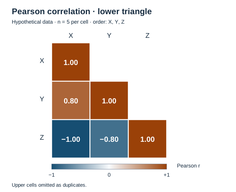
Reordering variables can bring related groups together. State the ordering or clustering method if you do this, and keep labels attached to the correct rows and columns. A cluster of similar colors is a prompt to investigate, not a causal explanation.
Pearson and Spearman matrices answer different questions
| Question | Pearson | Spearman |
|---|---|---|
| Association measured | Linear | Monotonic, through ranks |
| Values used | Original measurements | Ranks, usually averaging ties |
| Outlier sensitivity | Extreme values can dominate | Extreme magnitudes have less influence, but changed ordering still matters |
| Normality needed for calculation? | No | No |
| Detects every relationship? | No | No |
Choose according to the question, measurement scale and observed pattern. Pearson describes straight-line association between measured quantities. Spearman can describe whether higher ordered values tend to accompany higher or lower values, even along a monotonic curve. Neither adequately summarizes every U-shaped pattern.
For complete data, Spearman is Pearson correlation applied to consistently ranked columns [3]. In our example, each column already contains the ranks 1 through 5 in some order, so both matrices match. That agreement is specific to this dataset.
A rejected normality test does not automatically require Spearman. Tests and confidence intervals add assumptions beyond calculating a coefficient. See Pearson versus Spearman for a fuller method comparison.
Prepare the data before choosing missing-value handling
Check that each row refers to the same person, event or measurement across columns. Sorting columns independently destroys the pairing. Inspect coding and units; a postcode stored as a number is not automatically a quantitative measurement. Ordered response categories need a meaningful ordering.
Identify constant columns, missing values and unusual observations. Repeated measurements from one person and time-ordered records need attention to dependence. A computed coefficient does not make independent-observation inference appropriate.
Listwise deletion uses a common set of rows
Keep only observations complete across all selected variables. Every coefficient then uses the same retained sample. This makes comparisons easier, but can discard many records. If excluded observations differ systematically, the retained group may not represent the group you meant to study.
Pairwise deletion uses available pairs separately
Each cell uses rows with both relevant values present. The X–Y sample may differ from X–Z, so display a companion matrix of pair counts. A larger coefficient in one cell can reflect a different subset as well as a different relationship.
Neither deletion rule is universally unbiased. Do not replace blanks automatically with zero or column means; those choices can distort association. A justified imputation strategy depends on the missingness and analysis. Our missing-data guide covers the decision more broadly.
For Spearman with incomplete observations, check when software ranks the values. R documents reranking within each available pair for its pairwise option [3]. The Python example below removes incomplete rows first, so all ranks describe the same retained observations.
Why matrix validity matters
Values between −1 and +1 and a diagonal of ones are not enough to guarantee a coherent matrix. The entries must also fit together. Positive semidefinite means, in this setting, that the matrix does not imply a negative variance for any weighted combination of standardized variables.
A Pearson matrix from the same complete observations has this property, apart from numerical precision. So does Spearman calculated from consistently ranked complete columns. Pairwise deletion can break it [3]; inconsistent construction or aggressive rounding can also cause problems for downstream methods.
A valid matrix can still be singular, meaning some information is exactly redundant. Our example is singular because Z = 6 − X. This is a property of the data, not a computation error. Keep full precision for further analysis.
Correlation matrix versus covariance matrix
| Feature | Correlation | Covariance |
|---|---|---|
| Diagonal | 1 when defined | Variable variances |
| Units | Unitless | Products of variable units |
| Off-diagonal bounds | −1 to +1 for standard coefficients | No universal fixed bounds |
| Typical use | Compare association across pairs | Describe variability on original scales |
For Pearson, rᵢⱼ = covariance(Xᵢ, Xⱼ) ÷ [SD(Xᵢ) × SD(Xⱼ)]. Both standard deviations must be nonzero. Using sample covariance and sample standard deviations consistently cancels the common divisor. Spearman instead standardizes association between ranks, not the original measurements.
Create a correlation matrix in Python
This pandas workflow selects the intended columns and uses listwise deletion explicitly. pandas otherwise computes correlations from available pairs [4]. The two-observation minimum is a computational floor, not a claim that two observations support a useful estimate.
import pandas as pd

frame = pd.DataFrame({
    "X": [1, 2, 3, 4, 5],
    "Y": [2, 1, 4, 3, 5],
    "Z": [5, 4, 3, 2, 1],
})
selected = frame.loc[:, ["X", "Y", "Z"]]
complete = selected.dropna(axis=0, how="any")
pearson = complete.corr(method="pearson", min_periods=2,
                        numeric_only=False)
spearman = complete.corr(method="spearman", min_periods=2,
                         numeric_only=False)
print(pearson.round(2))
print(spearman.round(2))
Both printed matrices have these values. Rounding affects display only:
     X    Y    Z
X  1.0  0.8 -1.0
Y  0.8  1.0 -0.8
Z -1.0 -0.8  1.0
With seaborn and Matplotlib installed, add this heatmap. Explicit limits prevent the palette from rescaling to the observed range [5]:
import matplotlib.pyplot as plt
import seaborn as sns

fig, ax = plt.subplots(figsize=(6, 5))
ax.set_facecolor("#d1d5db")  # undefined cells are gray
sns.heatmap(pearson, vmin=-1, vmax=1, center=0,
            cmap="RdBu_r", annot=True, fmt=".2f",
            square=True, linewidths=1,
            cbar_kws={"label": "Pearson r"}, ax=ax)
for row in range(len(pearson)):
    for col in range(len(pearson.columns)):
        if pd.isna(pearson.iloc[row, col]):
            ax.text(col + .5, row + .5, "NA",
                    ha="center", va="center", color="black")
ax.set_title(f"Pearson correlation; n = {len(complete)}")
fig.tight_layout()
fig.savefig("correlation-heatmap.svg")
plt.close(fig)
Tested with pandas 2.2.3, seaborn 0.13.2 and Matplotlib 3.10.8. For one pair at a time, use the correlation calculator; this article's code supplies the complete matrix workflow.
Uncertainty, multiple testing and correlated predictors
A correlation matrix is not automatically a significance matrix. A large coefficient alone does not establish statistical significance, and a small p-value does not establish practical importance. Precision depends on sample size and study design. The five-row example reports descriptive coefficients only.
Ten variables create 45 distinct pairs. Testing every pair creates a multiple-testing problem. Choose a multiplicity strategy that matches the intended claims; procedures can control family-wise error or false discovery rate [6]. Significance stars need a named test, assumptions, sample sizes, handling of missing values and ties, and a statement about adjustment.
For regression, highly associated predictors deserve inspection. Multicollinearity concerns relationships among predictors in a model, including dependence involving several variables. Low pairwise correlations do not rule it out [7]. A cutoff such as 0.80 or 0.90 is not an automatic instruction to delete a column.
Use subject knowledge and the model's purpose to decide how to handle redundancy. Low marginal correlation with an outcome does not prove a predictor is useless: interactions and nonlinear effects may be missed. In machine learning, keep preprocessing and feature selection within training data and training folds; do not choose features using held-out test outcomes [8].
Common interpretation mistakes
- Calling a negative coefficient weak because it is negative, or treating zero as proof of no relationship.
- Reading heatmap color as significance and ignoring the number of pairs.
- Comparing cells from different subsets without qualification.
- Treating arbitrary numeric category codes as measurements.
- Confusing correlation with a regression slope or an adjusted effect. Partial correlation is a separate analysis.
- Deleting predictors by a fixed cutoff while ignoring the model.
- Overlooking outliers, clusters, repeated measurements or time trends.
- Claiming causation from association. Confounding and reverse causation remain possible.
Even a perfect sample correlation does not establish a causal mechanism. The guide to correlation versus causation explains that distinction.
A practical reading checklist
Identify the variables and units, then check the method, missing-data rule and pair counts. Read the sign and magnitude. Plot the pairs that matter, looking for unusual points, groups or curves. Consider uncertainty and study design before turning a descriptive result into a recommendation.
Frequently asked questions
What does a correlation matrix show?
It shows pairwise associations among several variables using a stated correlation method. Each cell summarizes one pair.
Why is the diagonal usually 1?
A varying variable correlates perfectly with itself. Constant variables or insufficient usable observations can make that self-correlation undefined.
Why is a correlation matrix symmetric?
Switching the order of two variables does not change their standard correlation when the observations and method stay the same.
How should I interpret negative values?
They indicate opposite-direction association of the type measured. Use absolute magnitude to assess its size, with context.
What is the difference between a matrix and a heatmap?
The matrix holds numbers. The heatmap encodes those numbers as colors; annotations or a companion table preserve exact values.
Should I choose Pearson or Spearman?
Choose Pearson for linear association in numerical measurements, or Spearman for monotonic rank association. Inspect the data and define the question first.
How do missing values affect the matrix?
They change which observations enter each coefficient. Pairwise deletion can produce different sample sizes and a matrix unsuitable for some later calculations.
Should I remove a highly correlated predictor?
Not automatically. Assess its role, redundancy and the model's purpose. Pairwise correlation alone cannot settle feature selection.
How does a covariance matrix differ?
Covariance keeps the measurement scales and has variances on the diagonal. Pearson correlation divides covariances by the corresponding standard deviations.
Does a correlation matrix show causation?
No. A matrix summarizes observed associations without identifying what would happen if you intervened on a variable.
References
- NIST/SEMATECH: scatter plots.
- SciPy: Pearson correlation, constant inputs and inference.
- R stats: correlation, covariance and missing observations.
- pandas: DataFrame.corr.
- seaborn: heatmap parameters.
- R stats: multiple-comparison adjustments.
- Purdue STAT 512: multicollinearity and limits of pairwise correlations, pages 10–12.
- scikit-learn: feature selection and data leakage.