
To interpret a scatter plot, read the axis labels and identify what each observation represents. Look for an upward or downward direction, then check whether the pattern is straight, curved or irregular. Judge how closely the points follow that pattern. Investigate unusual observations, separated groups and changes in spread before relying on a correlation coefficient or trendline. Describe the relationship using the variables and units shown, and limit your conclusion to the data collected. A visible association can help you ask better questions or build a model, but the chart alone does not establish cause and effect.
This guide explains how to interpret a scatter plot through worked examples, original diagrams and short practice questions. It belongs to AmriData’s Data Visualization guides. If you need the basic chart definition first, read what a scatter plot is.
How to interpret a scatter plot in 6 steps
| Step | Question to ask | Example finding |
|---|---|---|
| 1. Read the axes | What do X and Y measure? | Study hours and score units |
| 2. Identify direction | Does Y tend to rise or fall as X increases? | An upward tendency |
| 3. Examine form | Is the pattern straight, curved or irregular? | Approximately linear |
| 4. Evaluate strength | How closely do points follow the pattern? | A clear but imperfect association |
| 5. Check unusual features | Are there outliers, groups, gaps or changing spread? | One observation far from the others |
| 6. Add context | What conclusion does the sample support? | An association within five observations |
After reading the axes, use this memory aid: direction → form → strength → unusual features → context. Keep the actual points in view while reading any statistics printed beside them.
Step 1: Identify the X and Y variables
The horizontal X-axis gives one measurement; the vertical Y-axis gives the paired measurement for the same observation. A point at (3, 5) could mean three study hours and a score of five, or three thousand dollars spent and five thousand dollars earned. The labels decide which interpretation is valid.
Before describing the trend, establish the units, measurement period, sample size and population. Find out whether each point represents a person, store, country or day. Fifty daily measurements from one store are not equivalent to fifty independently sampled stores. Repeated observations can carry information about the same underlying subject.
X often contains an explanatory variable and Y an outcome. That arrangement does not assign a causal role. A chart can place either of two related measurements on the horizontal axis simply for convenience.
Check numerical spacing. On a linear axis, the distance from 2 to 10 must be eight times the distance from 1 to 2. Equally spacing those three values as category labels would distort the picture. A logarithmic axis follows a different rule: equal distances represent equal ratios. Read its tick labels before interpreting a curve or slope.
Count records rather than visible dots when possible. Several observations can have identical coordinates and overlap. A small sample also limits what you can learn: five tightly arranged points can produce a large correlation, yet leave considerable uncertainty about a wider population. A larger sample helps precision only when the collection process supports the question being asked.
Step 2: Identify the direction of the relationship
Read from left to right, following increasing X. A positive association means larger X values tend to occur with larger Y values. A negative association means larger X values tend to occur with smaller Y values. Individual points can depart from either trend.
In a study-hours example, an upward tendency means students with more recorded study hours tended to have higher scores in that sample. It does not mean every student who studied longer scored higher. For prices and quantities sold, a downward tendency would describe lower sales quantities at higher prices in the observed data; product differences and other factors still need investigation.
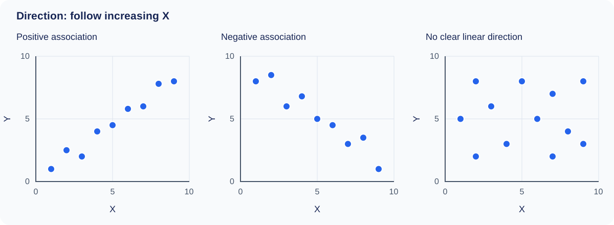
An irregular cloud may have no clear linear direction. That observation does not prove the variables are independent. Look for curves, subgroups or differences in variability before concluding that the chart contains little information.
Direction and strength answer different questions. A weak positive association and a strong positive association share the same sign. Swapping X and Y keeps Pearson’s correlation unchanged for the same pairs, but changes the question answered by a regression. The fitted slopes generally are not reciprocals of each other.
Step 3: Identify whether the pattern is linear or nonlinear
Form is the shape followed by the points. An approximately straight band suggests a linear summary may be useful. A curve calls for a description of where it rises, falls or levels off. For example, a saturation pattern rises quickly at first, then changes less at larger X values.
A monotonic pattern keeps the same overall direction across the range. An increasing curve can be monotonic without being straight. A U-shaped pattern is nonmonotonic: Y falls and then rises. Calling the entire U-shape positive or negative loses half its behavior.
A strong curve with Pearson r = 0
Consider the synthetic pairs (−2, 4), (−1, 1), (0, 0), (1, 1) and (2, 4). Every point lies exactly on Y = X². There is a perfect deterministic relationship in these five pairs, yet their Pearson correlation is exactly zero. The upward and downward parts balance in the calculation of linear association.
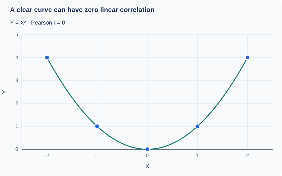
The correct description is “a U-shaped relationship, with the lowest Y at X = 0.” Saying “no relationship because r = 0” contradicts the plotted coordinates. Look at form before deciding whether a linear coefficient answers your question. NIST’s scatter plot handbook includes nonlinear patterns among the structures a scatter plot can reveal.
Step 4: Evaluate the strength of the association
Ask how consistently Y follows the form you identified. Points concentrated around a straight path suggest a strong linear association. A wide cloud with only a slight tilt suggests a weak linear association. For a curve, judge concentration around the curve rather than around an imaginary straight line.
Words such as weak, moderate and strong are approximate descriptions. There is no universal coefficient threshold that makes an association useful. A modest association may matter for a population-level question, while the same amount of scatter may be unacceptable for an individual prediction requiring high precision.
Do not judge strength by steepness. Changing hours to minutes makes a fitted slope numerically smaller without weakening the association. Stretching the chart vertically also makes the pattern look steeper without changing the underlying data or Pearson r. Compare plots with consistent scales and dimensions when you can.
Visual strength is not statistical significance. Population uncertainty depends on sample size, sampling design and model assumptions. Measurement reliability and the range of X also affect the observed relationship. A plot restricted to students studying four to five hours may look quite different from one covering zero to ten hours. That difference need not mean either chart was calculated incorrectly.
Step 5: Check outliers, clusters and changes in spread
Outliers, leverage and influence
An outlier is unusual relative to the pattern under study. A point far above a fitted line has a large positive residual: its observed Y exceeds its fitted Y. A point far along the X-axis can have high leverage, meaning it occupies an unusual predictor position. It may still lie close to the fitted line.
Influence describes how much a fitted result changes because of an observation. A point can alter the slope, correlation or R² substantially. Neither a large residual nor high leverage is a complete measure of influence on its own.
Check the original record before changing anything. An unusual value could be a typing error, a valid rare case or a member of another process. If it is valid, deleting it just to improve the correlation misrepresents the data. Report a sensitivity comparison when useful, explain any exclusion and retain the original analysis.
Groups, gaps and overlapping points
Separate clusters may correspond to regions, conditions or periods. Add known group labels and compare patterns within each group. Do not invent group identities from the arrangement alone. A gap could reflect limited sampling, eligibility rules or simply a small dataset.
Dense areas can hide observations. Transparency, smaller marks, count labels or density displays can reveal concentration. Jitter slightly offsets plotted positions to separate overlaps; disclose it when used and calculate statistics from the original coordinates. Rounding can also produce horizontal or vertical bands without implying distinct populations.
Changing spread
A funnel-shaped pattern suggests that the variability of Y may change with X. Suppose small stores have tightly clustered revenues while large stores show a wider range. The average trend may still rise, but a single prediction interval of fixed width could describe the data poorly.
In a regression model, heteroscedasticity means error variability is not constant. A widening band can suggest this issue; a residual plot helps assess it after fitting the mean pattern. An incorrect curve can also create apparent structure in residuals, so a funnel in the original scatter alone does not settle the diagnosis. Investigating these features is part of exploratory data analysis.
Step 6: Explain what the relationship means in context
Name the variables and the observations represented. “Higher advertising spending was associated with higher sales among the sampled campaigns” describes a finding. It leaves room for other explanations: higher demand could increase both spending and sales, and higher sales could allow a business to spend more.
Selection matters too. A chart containing only successful stores cannot automatically describe stores that closed. Poor measurement can change the shape and coefficient. Removing incomplete X–Y pairs can change the mix of observations if missingness is related to the variables. Record how many pairs were excluded and consult the guide to handling missing data before treating the remaining sample as equivalent to the original one.
Distinguish observational evidence from experimental evidence. A causal claim requires a defensible design and analysis that address alternative explanations. Even an experiment needs attention to assignment, adherence and measurement. A scatter plot is a display of the resulting data; it cannot supply those missing design details. See statistical analysis for the broader role of estimation and uncertainty.
Worked example: study hours and scores
The following five observations are synthetic data for learning. Scores use an illustrative numeric scale, not percentages. No real student outcomes are being reported.
| Observation | X: hours studied | Y: score units |
|---|---|---|
| A | 1 | 2 |
| B | 2 | 4 |
| C | 3 | 5 |
| D | 4 | 4 |
| E | 5 | 5 |
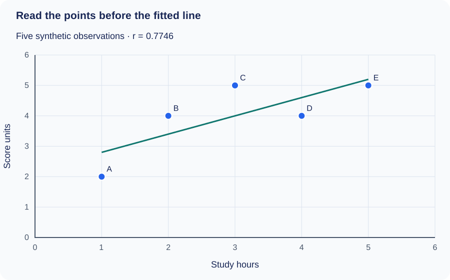
Direction is positive overall, although the score falls from 5 to 4 between three and four hours. The form is compatible with an approximate straight-line summary over this short range. The pattern is fairly clear but imperfect; five points provide little basis for judging its population stability. No observation is obviously isolated from the rest.
A complete interpretation could read: “Across these five synthetic observations, longer study time is associated with higher scores. The pattern is approximately linear with noticeable departures from the fitted line. Pearson r is about 0.775. The small illustrative dataset describes an association and does not establish that additional study time caused a score increase.”
Check the calculation
The mean X is 3 and the mean Y is 4. The sum of squared X deviations is 10, the sum of squared Y deviations is 6 and the sum of paired deviation products is 6. Therefore r = 6 / √(10 × 6) ≈ 0.7746. The least-squares slope is 6 / 10 = 0.6, and the intercept is 4 − 0.6 × 3 = 2.2.
These calculations use the actual coordinate pairs. They would be wrong if the X and Y columns were independently sorted, since that would break the pairing between each study time and its score.
How to interpret a scatter plot trendline and R²
A least-squares regression line summarizes a linear pattern by minimizing squared vertical residuals. In the example, ŷ = 2.2 + 0.6X. The hat on ŷ marks a fitted value. The slope means that each additional hour corresponds to an increase of 0.6 score units in the fitted value, within this model.
At X = 4, the fitted score is 4.6. Observation D has an actual score of 4, so its residual is 4 − 4.6 = −0.6. Residuals retain information the line hides. A curved residual pattern suggests a straight line has missed the mean structure; a widening residual band suggests changing variability.
The intercept, 2.2, is the model’s fitted score at zero hours. Zero lies outside the observed one-to-five-hour range. The intercept is needed to position the line, but these data do not establish what actually happens at zero hours. Predicting at ten hours would be a much larger extrapolation. An apparently sensible formula can give unreliable answers beyond the measurements used to fit it.
For this ordinary least-squares regression with one predictor and an intercept, R² = r² = 0.60. The residual sum of squares is 2.4 and the total sum of squared score deviations from the mean is 6, giving R² = 1 − 2.4/6. The fitted line accounts for 60% of that sample’s squared variation around its mean.
It does not mean 60% of scores are correct, that every prediction is 60% accurate or that study time causes 60% of performance. R² also loses direction: a negative slope can have a high R². The equality R² = r² applies to the stated simple regression setup, not to every model called a trendline. No-intercept fits and evaluation on new observations require additional care.
A high in-sample R² does not guarantee useful prediction on new data. Check residual size in the original units, inspect model assumptions and assess performance on observations not used for fitting when prediction is the goal.
How one unusual point changes the result
Add a sixth synthetic observation, F = (10, 1), to the study-hours example. It is far beyond the other X values and below their upward trend. Both the coefficient and fitted line change markedly:
| Dataset | Pearson r | Fitted line | R² |
|---|---|---|---|
| Original five pairs | 0.7746 | ŷ = 2.2000 + 0.6000X | 0.6000 |
| With F = (10, 1) | −0.4390 | ŷ = 4.4426 − 0.2262X | 0.1927 |
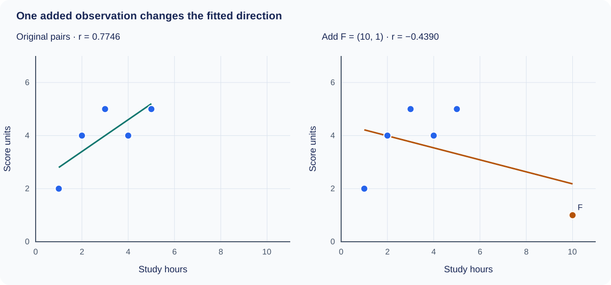
The numerical reversal is a reason to investigate F, not a reason to discard it. If it is a recording error, correct it using the source. If it is valid, ask whether one line describes all six observations adequately and report the sensitivity of the conclusion. The example shows why quoting only the final correlation would hide important structure.
When pooled data hide the group pattern
Consider another synthetic dataset. Group A contains (1, 8), (2, 9), (3, 10). Group B contains (4, 2), (5, 3), (6, 4). Within each group, Y rises exactly one unit per unit of X, so each within-group correlation is +1. Across all six points, Pearson r is approximately −0.722.
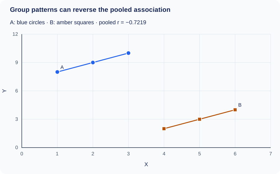
This is a grouped-data reversal, often discussed under Simpson’s paradox. The groups occupy different X ranges and different Y levels. An overall downward trend therefore answers a different question from either within-group trend.
In real data, examine what the group variable means before deciding whether to combine, stratify or adjust. Do not automatically prefer the pooled or separated result. The research question and causal structure determine which comparison is meaningful. Here, three exact points per group illustrate the arithmetic; they provide no real-world evidence about stability or cause.
Common scatter plot interpretation mistakes
| Mistake | Better interpretation |
|---|---|
| “The steepest line is the strongest relationship.” | Check dispersion and units. Slope measures fitted change, not strength. |
| “Zero correlation means no relationship.” | Look for curves and subgroup structure. |
| “The outlier must be wrong.” | Check the source and the process that produced it. |
| “R² measures prediction accuracy as a percentage.” | Describe the model’s squared variation measure and inspect prediction errors. |
| “The trend will continue beyond the chart.” | Identify extrapolation and seek observations in that range. |
| “Every visible dot is one independent case.” | Check overlapping coordinates and repeated measurements. |
Scatter plot axes do not always need to start at zero. A restricted axis can help show variation, provided its scale is clear and points are not selectively hidden. Compare the labels and limits rather than treating a cropped axis as automatically dishonest. Aspect ratio, reversed scales and log transformations can all change visual appearance.
Connecting unrelated observations in row order adds a path the data may not justify. If the question concerns change through ordered dates, a line graph may be more appropriate. Use the guide to choosing a chart type for that decision, and the guide to data visualization mistakes for broader presentation checks.
How to write a scatter plot conclusion
Begin with what was measured and what the points show. Add the range, sample size or grouping when they affect the claim. Use a coefficient only after checking that its type matches the pattern.
The scatter plot shows a [direction] association between [X, with units] and [Y, with units] among [observations]. The pattern is approximately [form], with [description of strength and unusual features]. Within the observed range, larger X values tend to accompany [description of Y]. [Relevant sampling, measurement or model limitation] limits the conclusion.
Replace only the parts the chart supports. For the U-shape, describe the change in direction instead of forcing “positive” into the first sentence. For an irregular cloud, say “no clear pattern is visible in this sample” and mention whether overlapping points or a narrow range limit the assessment.
A report about the grouped example might say: “The pooled data show a negative association, but both labeled groups show positive within-group patterns. A single overall coefficient conceals this difference.” That statement is more informative than assigning one strength label to the full chart.
Practice interpreting three patterns
1. Points form a narrow downward band
What can you conclude? Describe a strong negative, approximately linear association over the plotted range. Larger X tends to accompany smaller Y. You still need variable names, units and sampling context to produce a complete interpretation. The negative sign does not mean the relationship is weak.
2. Points rise, then flatten
What should you inspect before reporting r? Check the curved form. A positive monotonic association with saturation may fit the visual pattern better than a constant linear slope. A straight-line model can systematically overpredict one region and underpredict another even when r is positive.
3. A trend appears only after combining groups
What is the next step? Identify the group variable and compare within-group plots on consistent axes. Check whether group membership explains differences in location. Do not conclude that changing X within a group will reproduce the pooled association.
Frequently asked questions
How do you interpret a scatter plot in one sentence?
Name the variables, describe the direction and form, qualify the strength and mention the feature that most affects interpretation. For example: “In these five synthetic pairs, study hours and scores have a positive, approximately linear association, with visible scatter and a sample too small for broad conclusions.”
What does a positive correlation scatter plot look like?
The points tend to rise from lower left to upper right as X increases. Some points can depart from that tendency. Check whether the rising form is approximately straight before interpreting Pearson r as its summary.
Can a scatter plot show a strong relationship with no correlation?
It can show a strong nonlinear relationship with zero Pearson correlation. The five-point Y = X² example above demonstrates this exactly. Specify “zero linear correlation” to avoid implying that the variables have no relationship.
Is a correlation of −0.9 weaker than +0.5?
No. In terms of Pearson linear association, −0.9 has the larger absolute magnitude. Its sign indicates a downward direction. Neither coefficient establishes cause or guarantees a useful individual prediction.
Should I remove outliers before fitting a trendline?
Investigate them first. Correct verified errors, document justified exclusions and examine how valid unusual observations affect the fit. Removing a record simply because it weakens the desired trend is not a defensible rule.
What if every Y value is identical?
The points form a horizontal row. Pearson r is undefined because Y has zero variance; it is not numerically zero. The usual centered R² also has a zero denominator. Software may display a warning, a special value or no statistic.
Does a high R² prove cause and effect?
No. R² summarizes fit under a specified calculation. Confounding, selection and reverse causation can remain even when the fitted line follows the data closely. A causal claim requires evidence about the study design and process.
Related guides
Sources and calculation notes
The diagrams and numerical examples in this guide are original synthetic teaching material. Correlations, least-squares coefficients and residual sums were calculated from the listed pairs. The following references support the general interpretation framework:
- NIST/SEMATECH e-Handbook: Scatter plot covers nonlinear structure, changing variation, outliers and the limits of causal interpretation.
- Khan Academy: Describing scatterplots introduces form, direction, strength and outliers.
- University of Texas: Scatterplot illustrates linearity, strength and unusual observations.
When interpreting your own scatter plot, write the contextual description before copying the coefficient into your report. Then check that the coefficient, chart and wording tell the same story.
← Back to Data Visualization