
A scatter plot shows how two numerical variables vary together. Each dot represents one observation, positioned by its X and Y values. Read the pattern to spot associations, curves, clusters and unusual records before reducing the data to a single statistic.
This article belongs to our Data Visualization guides. Start with five fictional students, then use the same observations to understand correlation and a fitted line.
What is a scatter plot?
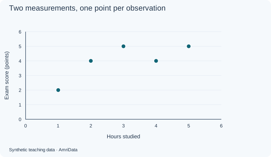
A scatter plot is a graph of two numerical measurements recorded for the same observations. Each dot has a horizontal position, X, and a vertical position, Y. A dot could represent a student, store, day or experimental unit. Looking across the dots reveals whether larger X values tend to accompany larger or smaller Y values, whether the pattern curves, and whether some observations stand apart. Scatter plots are also called scatter diagrams, scatter graphs or XY plots. They show associations in the recorded data; they do not establish what caused those associations.
| X | Y |
|---|---|
| 1 | 2 |
| 2 | 4 |
| 3 | 5 |
| 4 | 4 |
| 5 | 5 |
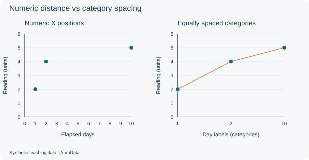
Coordinates matter. The point (3, 5) means X is 3 and Y is 5. On a linear horizontal scale, the gap from 2 to 10 must be eight times the gap from 1 to 2. Giving all three values equal spacing changes the picture. A scatter plot uses numerical positions on both axes, even when the values are whole numbers.
Scatter plot example: study hours and exam scores
Synthetic example created for teaching. These scores use an illustrative point scale, not percentages. Each row preserves one student's two measurements.
| Student | Hours studied (X) | Exam score (points, Y) |
|---|---|---|
| A | 1 | 2 |
| B | 2 | 4 |
| C | 3 | 5 |
| D | 4 | 4 |
| E | 5 | 5 |
Plot A one hour across and two points up. Plot B at (2, 4), C at (3, 5), D at (4, 4) and E at (5, 5). There are five records and five distinct dots. The overall pattern rises, although D's score is lower than C's. Positive association does not require every successive point to be higher.

| X | Y |
|---|---|
| 1 | 2 |
| 2 | 4 |
| 3 | 5 |
| 4 | 4 |
| 5 | 5 |
These five observations have mean study time 3 hours and mean score 4 points. Pearson correlation is approximately 0.7746. That describes a fairly strong positive linear association in this tiny teaching sample; it is not evidence that an extra hour guarantees a better score.
Parts of a scatter plot
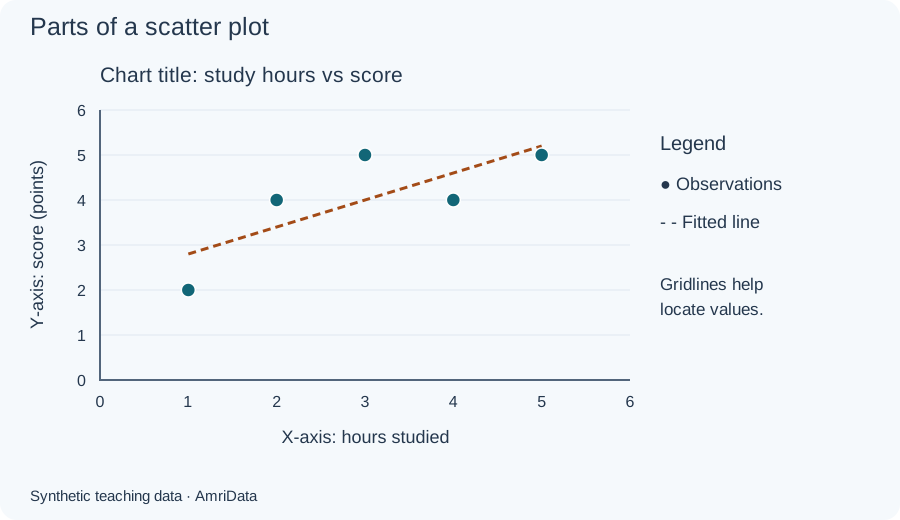
The X-axis runs horizontally. In a predictive analysis it often holds the explanatory variable. The Y-axis runs vertically and often holds the response. Assigning these roles does not establish causation. If the question is simply whether two measurements vary together, neither needs to be called independent or dependent.
| X | Y |
|---|---|
| 1 | 2 |
| 2 | 4 |
| 3 | 5 |
| 4 | 4 |
| 5 | 5 |
Give the chart a specific title and label both axes with variable names and units. “Hours studied” and “Exam score (points)” let readers interpret a dot without consulting the original spreadsheet. Light gridlines help locate values. A legend explains groups or distinguishes observations from an optional fitted line. Use marker shapes as well as colors when groups appear.
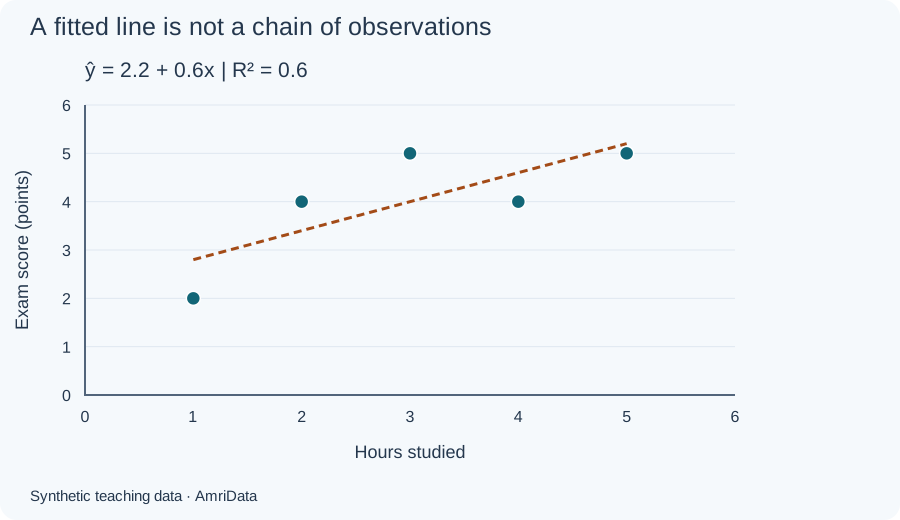
A trendline summarizes a model. It is separate from the observations and usually does not pass through every dot. Joining student A to B to C instead would imply a sequence that is irrelevant to this question.
Types of scatter plot patterns
These names describe patterns, not different chart formats. Examine direction, curvature and spread together. The numerical examples below are all synthetic; expand each figure's data disclosure to inspect every plotted pair.
Positive and negative linear association
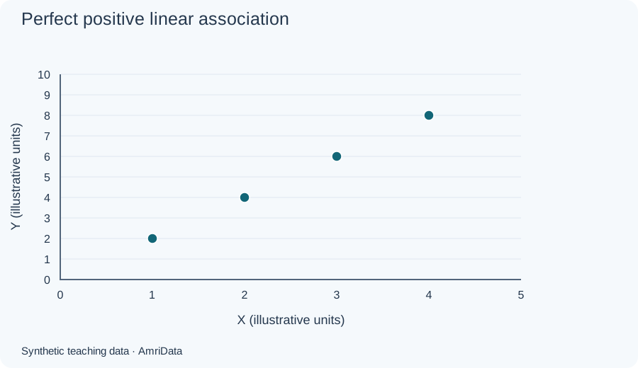
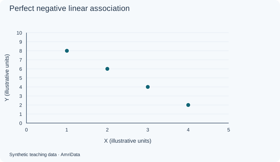
A positive pattern rises from left to right. A negative pattern falls. Perfect positive correlation occurs for (1, 2), (2, 4), (3, 6), (4, 8): every point lies on one rising straight line, so r = 1. The descending pairs (1, 8), (2, 6), (3, 4), (4, 2) give r = −1. Both are exact constructed examples, not typical measurement data.
| X | Y |
|---|---|
| 1 | 2 |
| 2 | 4 |
| 3 | 6 |
| 4 | 8 |
| X | Y |
|---|---|
| 1 | 8 |
| 2 | 6 |
| 3 | 4 |
| 4 | 2 |
Weak positive, weak negative and no linear association
When points are widely dispersed around a rising or falling direction, the linear association is weak. That description depends on the measurement context; there is no universal cutoff that makes every correlation “strong.” The weak examples here deliberately keep substantial variation around a slight direction.
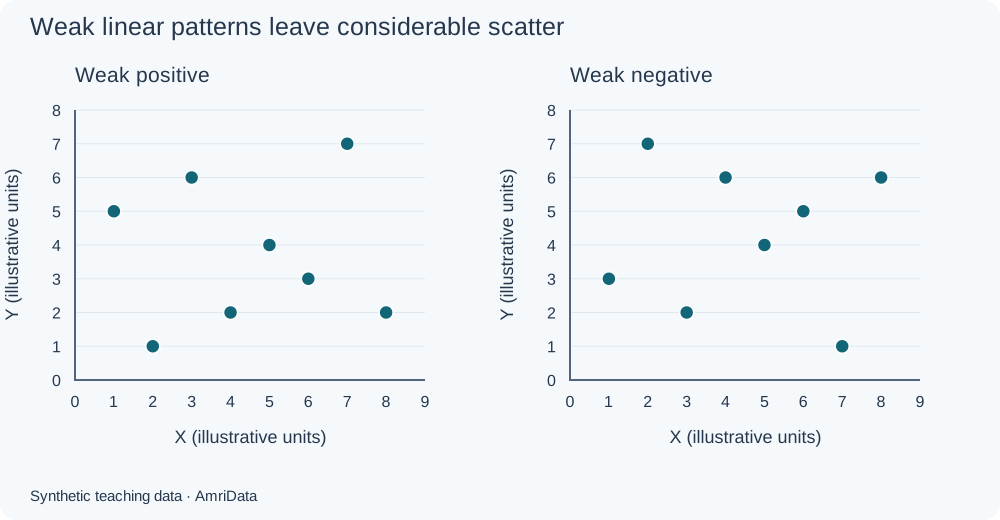
| X | Y |
|---|---|
| 1 | 5 |
| 2 | 1 |
| 3 | 6 |
| 4 | 2 |
| 5 | 4 |
| 6 | 3 |
| 7 | 7 |
| 8 | 2 |
| X | Y |
|---|---|
| 1 | 3 |
| 2 | 7 |
| 3 | 2 |
| 4 | 6 |
| 5 | 4 |
| 6 | 5 |
| 7 | 1 |
| 8 | 6 |
A cloud without an overall rising or falling direction may have little linear association. It can still contain subgroups, changing variability or other structure. Inspect the plotted values rather than treating a small correlation as permission to stop exploring.
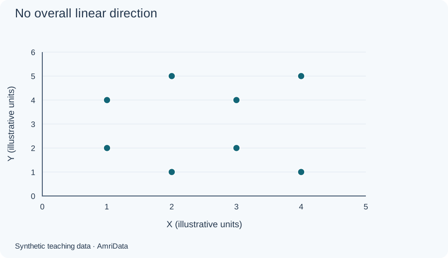
| X | Y |
|---|---|
| 1 | 2 |
| 1 | 4 |
| 2 | 1 |
| 2 | 5 |
| 3 | 2 |
| 3 | 4 |
| 4 | 1 |
| 4 | 5 |
A curved pattern can have zero Pearson correlation
Consider (−2, 4), (−1, 1), (0, 0), (1, 1), (2, 4). Every Y value equals X squared, giving an exact U shape. Yet Pearson r is zero because the negative and positive sides balance. Zero linear correlation therefore does not establish independence or the absence of a relationship.
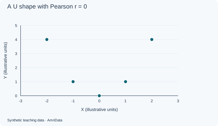
| X | Y |
|---|---|
| -2 | 4 |
| -1 | 1 |
| 0 | 0 |
| 1 | 1 |
| 2 | 4 |
Clusters, outliers and changing spread
Separated groups may reflect different products, regions or experimental conditions. Investigate their meaning before naming them. A combined upward pattern can mostly reflect differences between groups even when the association inside each group is weak or different. Plot meaningful groups separately when their sample sizes allow it.

| X | Y |
|---|---|
| 1 | 2 |
| 1.5 | 1.5 |
| 2 | 2.5 |
| 6 | 6.5 |
| 6.5 | 6 |
| 7 | 7 |
| 3 | 8 |
An outlier lies away from the main pattern. Check its source record, units and circumstances. It may be a transcription error, a separate population or a valid unusual result. Removing it merely because it weakens a preferred conclusion changes the evidence. Compare justified analyses with and without influential observations and explain the decision.
A widening funnel means the spread of Y increases across X. In regression, changing error variance is called heteroscedasticity; a scatter plot can flag a possible issue, while residual checks help assess the fitted model. These investigations fit into a broader exploratory data analysis.
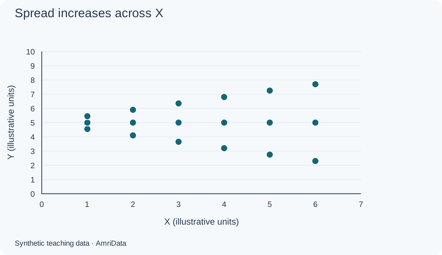
| X | Y |
|---|---|
| 1 | 4.55 |
| 1 | 5 |
| 1 | 5.45 |
| 2 | 4.1 |
| 2 | 5 |
| 2 | 5.9 |
| 3 | 3.65 |
| 3 | 5 |
| 3 | 6.35 |
| 4 | 3.2 |
| 4 | 5 |
| 4 | 6.8 |
| 5 | 2.75 |
| 5 | 5 |
| 5 | 7.25 |
| 6 | 2.3 |
| 6 | 5 |
| 6 | 7.7 |
| Pattern | What it suggests | Main caution |
|---|---|---|
| Positive or negative linear | A direction of association | No causal conclusion |
| Weak linear | Limited straight-line alignment | Other structure may remain |
| No linear direction | Little linear association | Check for curves |
| Curved | A nonlinear relationship | A straight fit may miss it |
| Clusters | Possible subgroups | Investigate group membership |
| Outlier | An unusual record | It may be valid |
| Funnel | Changing variability | Check model assumptions |
How to read a scatter plot
Use this sequence: direction → form → strength → unusual features → context.
- Direction: Does Y generally rise or fall as X increases?
- Form: Is the relationship approximately straight, curved or split into groups?
- Strength: How closely do the points follow that form? A tight curve can be strong even with low Pearson r.
- Unusual features: Look for gaps, repeated coordinates, isolated points and widening spread.
- Context: Identify units, collection method, sample size, selection rules and what each dot represents.
For our students: “The five scores generally increase with study hours, with departures from a straight-line pattern. Scores at three and four hours interrupt a strictly increasing sequence. This small fictional sample illustrates association; it cannot support a population or causal conclusion.” That statement explains both the visible finding and its limits.
Scatter plots and correlation
Pearson's r measures the direction and strength of linear association. When defined, it falls between −1 and 1. Its sign gives direction; its magnitude describes straight-line alignment. Swapping X and Y leaves r unchanged, but changes which variable a regression predicts. A scatter plot also reveals shapes that this single number cannot capture.
If either variable is constant, r is undefined, not zero. Extreme observations can change r substantially. With very few observations, even a large absolute r is weak grounds for general claims. Spearman correlation uses ranks to summarize monotonic association; it also cannot replace inspecting the graph.
Check the correlation calculationUsing x̄ and ȳ for sample means, r = Σ[(x − x̄)(y − ȳ)] ÷ √[Σ(x − x̄)² × Σ(y − ȳ)²]. For the five students, x̄ = 3, ȳ = 4, the cross-product sum is 6, and the squared-deviation sums are 10 and 6. Therefore r = 6 ÷ √60 = 0.7745966692.
For further interpretation, see Berkeley's discussion of correlation and association and our statistical analysis guide.
Correlation does not prove causation
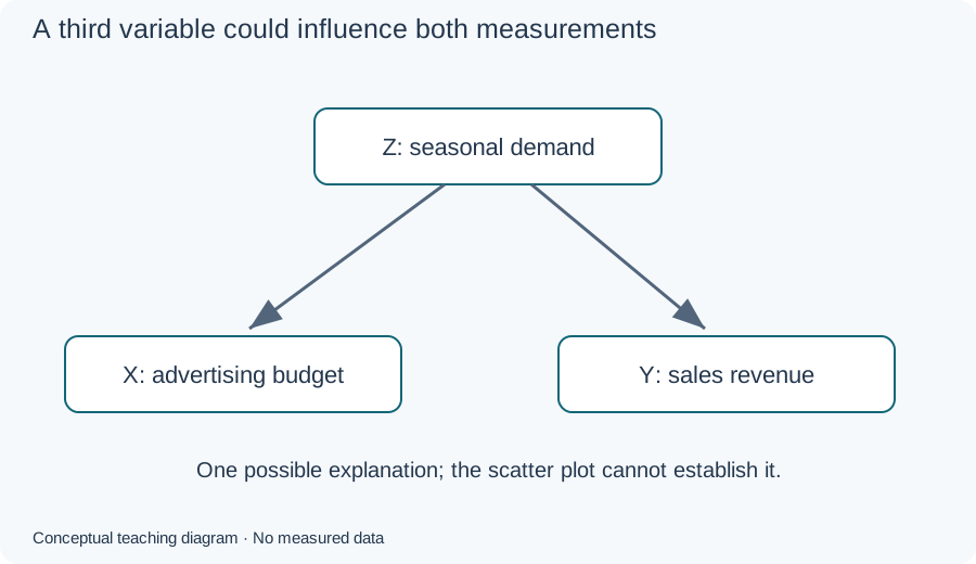
An association might involve X influencing Y, Y influencing X, a shared cause, selection effects or chance. For example, seasonal demand could influence both advertising budgets and sales. A scatter plot of spending against sales cannot separate those possibilities. A suitable study design and additional evidence are needed to investigate causal effects.
What is a line of best fit?
An ordinary least-squares regression line predicts Y from X by minimizing squared vertical residuals. A residual is the observed Y minus the fitted Y at that X. The equation is ŷ = a + bx, where a is the intercept, b is the slope and ŷ is the predicted value.
| X | Y |
|---|---|
| 1 | 2 |
| 2 | 4 |
| 3 | 5 |
| 4 | 4 |
| 5 | 5 |
For our five students, ŷ = 2.2 + 0.6x. An extra hour is associated with a 0.6-point increase in the fitted score. At three hours, the line predicts 4 points, while student C actually scored 5. The residual is therefore 1 point. The intercept predicts 2.2 points at zero hours, outside the observed one-to-five-hour range; it need not have a useful practical interpretation.
What does R² mean?
For this fit, the squared residuals total 2.4 and the squared deviations from the mean score total 6. Thus R² = 1 − 2.4/6 = 0.6. The line accounts for 60% of the observed score variation under the centered sample definition. It does not mean that study hours caused 60% of performance or that predictions are 60% accurate.
In ordinary simple linear regression with an intercept and nonconstant variables, R² equals r². Do not apply that identity to every regression method. A high R² can coexist with a misleading model, influential observations or poor predictions on new data. Penn State's correlation and regression lesson develops these concepts further.
A straight line is a poor summary of pronounced curvature or conflicting group patterns. Inspect residuals before using a model for inference. Extending the student line to 20 hours would be extrapolation far beyond the observations, with no evidence here that the relationship persists.
How to make a scatter plot step by step
- Choose two numerical measurements that answer a relationship question.
- Keep paired values in the same row, with a record identifier if needed.
- Check units, numeric types, missing values and possible recording errors.
- Assign X horizontally and Y vertically; choose readable numeric scales.
- Plot one marker per complete observation at its exact coordinates.
- Add a descriptive title and axis names with units.
- Inspect the pattern before adding an optional model line.
Never sort X and Y independently. Doing so destroys the original pairs and can manufacture an association. If one measurement is missing, the pair cannot be positioned on an ordinary two-variable scatter plot. Report excluded counts and consider whether exclusions change the represented population. See how to handle missing data; an unknown value is not automatically zero.
Repeated coordinates are legitimate. Two students with the same hours and score may appear as one dot. Transparency, smaller markers, count labels or a documented small jitter can reveal overlap. Jitter changes displayed positions, so retain exact values in a table and disclose the adjustment. For dense datasets, consider a density or hexbin plot rather than hiding most observations behind opaque markers.
Choose honest axis ranges
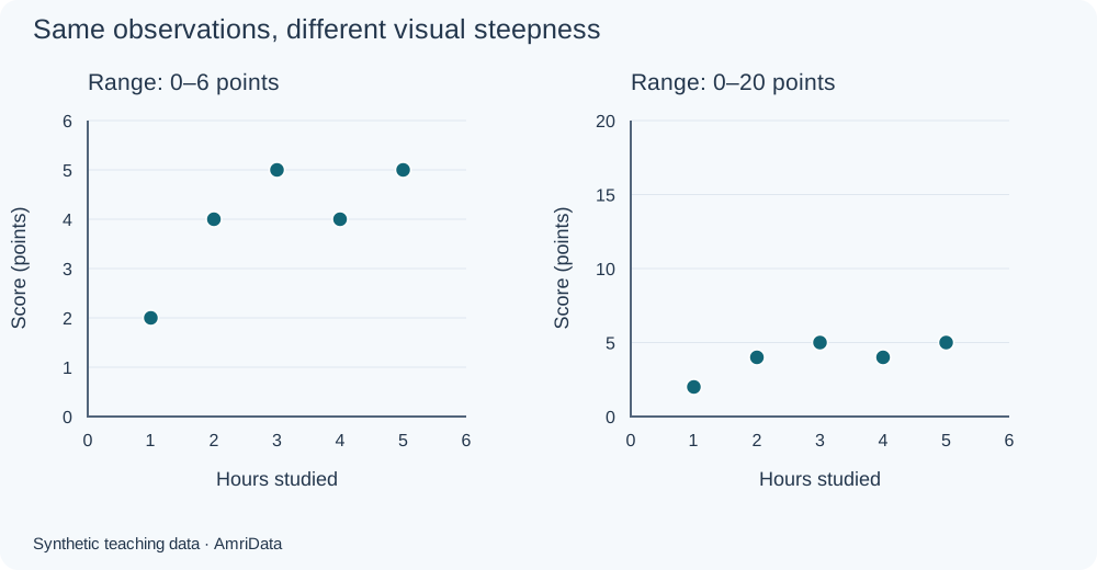
Scatter plot axes do not always have to start at zero. Clearly labeled ranges around the data can reveal differences. Changing axis ranges or the chart's aspect ratio changes apparent steepness, however. It does not change Pearson r for unchanged values. Logarithmic transformations are different: they change the numeric scale and may change correlation calculated on the transformed data.
| X | Y |
|---|---|
| 1 | 2 |
| 2 | 4 |
| 3 | 5 |
| 4 | 4 |
| 5 | 5 |
Make a scatter plot in Excel or Google Sheets
Excel
Enter “Hours studied” in A1 and “Exam score (points)” in B1, then put the five pairs in rows 2–6. Select A1:B6 and choose Insert → X Y Scatter, using markers only. Under Chart Design, use Add Chart Element for axis titles. Check the selected series uses A2:A6 for X and B2:B6 for Y.
For the optional linear fit, choose Chart Design → Add Chart Element → Trendline → Linear. Trendline formatting offers equation and R² labels in supported desktop versions. Keep the fitted intercept free for this example. Menu placement varies by version; use Microsoft's scatter-chart instructions and trendline guidance.
Check that numbers were not imported as text or dates, X and Y were not swapped, and blanks were handled deliberately. A standard line chart can treat numeric labels as equally spaced categories, which is unsuitable when actual X distances matter.
Google Sheets
Use the same two-column layout. Select the table, choose Insert → Chart, and set the chart type to Scatter chart. In Chart editor → Setup, check the X-axis and Y series. Under Customize, edit Chart & axis titles and Series; a trendline is optional. Review the official scatter-chart guide for data layout and trendline settings for the fitted line.
Make a scatter plot online
The same checks apply in an online chart maker: enter paired numeric values, confirm axis assignments, count the plotted records and inspect labels before exporting. If importing CSV, inspect the preview for delimiters and number formats. Check the interface for supported download formats. You can browse AmriData's free chart and data tools for available options.
When should you use a scatter plot?
Use one when your question concerns two quantitative measurements on the same units. It is particularly useful early in an investigation, before a correlation coefficient or model hides the individual observations. For broader selection advice, see how to choose a chart type.
| Setting | X and Y | What to investigate |
|---|---|---|
| Education | Study hours and score | Prior preparation and course differences |
| Business | Advertising spend and sales | Seasonality and budget allocation |
| Ecommerce | Price and units sold | Category, brand and product age |
| Health research | Age and blood pressure | Other factors and sampling; no clinical rule implied |
| Environment | Temperature and electricity demand | Possible heating and cooling curves |
| Experiment | Concentration and measured response | Curvature and unusual measurements |
| Business reporting | Revenue growth and profitability | Consistent definitions and accounting periods |
| Marketing | Impressions and conversions | Campaign size and audience differences |
Scatter plot vs line graph and other charts
A scatter plot asks how two numerical variables relate. A line graph usually follows a measurement through a meaningful order, often time. Some line charts use continuous date axes; others space category labels equally. An XY chart can connect points when a trajectory matters, but connecting unrelated observations adds an unsupported sequence.
| X | Y |
|---|---|
| 1 | 2 |
| 2 | 4 |
| 10 | 5 |
For a time-based report, see how to make a line graph or the Line Graph Maker. Preserve actual time gaps when they matter to the interpretation.
| Chart | Main purpose | Difference from a scatter plot |
|---|---|---|
| Bar chart | Compare categories | Category positions are not numeric X measurements |
| Histogram | Show one variable's distribution | Bins values instead of retaining X–Y pairs |
| Box plot | Summarize median, quartiles and spread | Does not show each paired relationship |
| Bubble chart | Add a third numeric measurement | Encodes it using marker area; label the size scale |
| One-variable dot plot | Show individual values on one scale | “Dot plot” terminology varies; it need not mean XY |
If you need a distribution instead, try the Histogram Maker or read what a box plot shows. A correlation coefficient is a numerical summary, not a replacement chart.
Advantages and limitations
Scatter plots keep individual observations visible and can reveal curves, subgroups and unusual values that an average conceals. They require little calculation to read. Their usefulness depends on the measurements and sampling: an attractive pattern does not validate the records or reveal omitted units.
Large datasets can overlap, small samples can look persuasive by chance, and mixed groups can obscure different relationships. A plot alone does not establish statistical significance, independent observations or reliable forecasts. Use collection knowledge and suitable statistical checks alongside the picture.
Common scatter plot mistakes
| Mistake | Consequence | Correction |
|---|---|---|
| Equally spaced numeric labels | Distorts X distances | Use an XY numeric axis |
| Sort columns separately or swap assignments | Changes pairings or prediction meaning | Keep rows intact; verify the series |
| Connect unrelated dots | Invents a sequence | Use markers only |
| Omit titles, units or group legend | Makes values ambiguous | Name measurements and groups |
| Compress axes to hide variation | Changes the visual impression | Show readable ticks and deliberate ranges |
| Replace missing values with zero | Invents observations | Investigate and report exclusions |
| Delete repeated coordinates | Undercounts valid records | Check IDs and reveal overlap |
| Report r without plotting | Can conceal curvature or outliers | Inspect the graph first |
| Force a straight line on a curve | Misses the main relationship | Consider an appropriate model |
| Ignore outliers or subgroups | Lets a few records or group differences dominate | Investigate and compare justified analyses |
| Generalize from a tiny sample | Overstates evidence | Report sample and design limitations |
| Use opaque, oversized markers | Hides frequency and detail | Adjust markers or use density summaries |
| Call R² a causal percentage | Confuses fit with cause | Describe observed variation and assumptions |
| Extrapolate far beyond X | Assumes an unobserved pattern persists | Limit predictions and assess uncertainty |
| Assume the graph validates the data | Plausible errors remain unnoticed | Check records against source information |

| X | Y |
|---|---|
| 1 | 2 |
| 2 | 4 |
| 3 | 5 |
| 4 | 4 |
| 5 | 5 |
Frequently asked questions
What is a scatter plot?A graph that places paired numerical observations at their X and Y coordinates.
What does a scatter plot show?Direction, form, spread, clusters and unusual observations in paired measurements.
What is a scatter plot used for?Exploring relationships before choosing a summary, model or further investigation.
What is another name for a scatter plot?Scatter diagram, scatter graph and XY plot are common alternatives.
What are its main parts?Two numeric axes, paired observations, a title and axis labels; a legend or trendline may be added.
How do you read one?Check direction, form, strength, unusual features and the measurement context.
How do you make one?Keep two numeric columns paired by row, select an XY scatter chart and verify labels and scales.
What goes on the X-axis?One numerical measurement, often the explanatory or predictor variable.
What goes on the Y-axis?The paired numerical measurement, often the response or outcome.
What does each dot represent?One observation with both measurements, such as a store, student or day.
What is a positive scatter plot?A plot in which Y generally rises as X increases.
What is a negative scatter plot?A plot in which Y generally falls as X increases.
What does no correlation mean?For Pearson correlation, little or no straight-line association; other relationships may remain.
What is weak correlation?Limited linear alignment. The practical meaning depends on the field and measurements.
Can a scatter plot show a nonlinear relationship?Yes. A curve can be visible even when Pearson r equals zero.
What are the main patterns?Rising, falling, weak, curved, clustered and outlying patterns; spread can also change across X.
What does an outlier mean?A record is unusual relative to the pattern. Investigate before deciding whether it is erroneous.
What does a cluster mean?Several observations occupy a similar region. Their shared meaning needs investigation.
What is a line of best fit?A fitted summary of a relationship; ordinary least squares minimizes squared vertical residuals.
Does every plot need a trendline?No. Raw points may be sufficient, and a straight line can misrepresent a curve.
What does Pearson r mean?The direction and strength of linear association, on a scale from −1 to 1 when defined.
What does r = 0 mean?Zero measured linear association. It does not prove independence.
What does r = −1 mean?All observations lie on a straight line with a negative slope, with both variables nonconstant.
What does R² mean?For the ordinary fitted line here, the fraction of centered observed Y variation accounted for by the fit.
Does a scatter plot prove causation?No. Shared causes, reverse direction, selection and chance may explain an association.
Can X and Y be negative?Yes, if negative values are valid for the measurements. Show their actual coordinates.
Can two points have the same coordinates?Yes. Overlap may hide records; a matching position does not prove duplication.
Must the axes start at zero?No. Use clear numeric ticks and ranges appropriate to the question.
Can scatter plots show categories?Categories can distinguish marker groups. The ordinary X and Y positions still represent numerical measurements.
How does a scatter plot differ from a line graph?It usually emphasizes relationships between numeric pairs; a line graph usually emphasizes ordered progression.
How does it differ from a histogram?A histogram summarizes one variable in bins. A scatter plot retains two-variable pairs.
How does it differ from a bubble chart?A bubble chart adds a quantitative measurement through marker size, usually area.
Can I use Excel?Yes. Choose an XY scatter chart, check the series ranges and add axis titles.
Can I use Google Sheets?Yes. Select Scatter chart and check X-axis and series assignments in Setup.
Can I make one online for free?Online chart makers may offer free plotting. Check the selected tool’s current access and limits.
Can I upload CSV data?Only if the chosen maker supports import. Check paired columns, numeric types and missing records afterward.
How do I download the graph?Use the selected application’s export controls and check its supported formats and output labels.
When should I use another chart?Use a bar chart for category comparisons or a distribution chart for one numerical variable.
What to remember
What is a scatter plot useful for? Seeing the paired observations before deciding how to summarize them. Keep numeric distances accurate, read the shape and inspect unusual records. Use correlation and a fitted line when they suit that shape, and keep the conclusion within what the data and study design support.
Related Data Visualization guides and tools
Sources and further reading
The examples and charts on this page were created for teaching. For the statistical background, consult the NIST scatter plot reference, Penn State's descriptive statistics lesson, and the correlation and software references linked above.
← Back to Data Visualization guides