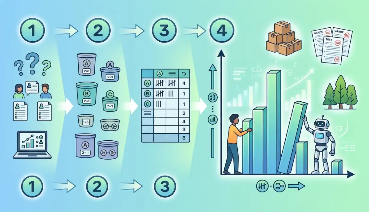
To make a histogram, start with numerical observations, divide their values into non-overlapping intervals called bins, and count how many observations belong to each interval. Draw a rectangle over each bin on a numerical x-axis. For equal-width bins, its height can show the count (frequency) or the percentage of observations. Label the axes and check that every observation is counted once. You can also make a histogram with AmriData, Excel, Google Sheets, Python or Matplotlib.
We will use the same 18 test scores throughout this guide. First we will build a histogram by hand, with a frequency table you can check. Then we will use the same numbers in five different chart-making workflows. You will also see why software output can look different when its automatic bin boundaries differ.
Part of AmriData's Data Visualization guides. For definitions, histogram shapes and how to read the finished chart, see the histogram explanation.
Jump to a method: By hand · AmriData · Excel · Google Sheets · Python/pandas · Matplotlib · FAQs
How to Make a Histogram in 7 Steps
- Collect numerical data. Use measurements or numerical counts, not names of categories.
- Find the minimum and maximum. Check the observed spread of the values.
- Choose sensible bins. Decide how many intervals to use and how wide they should be.
- Write the exact boundaries. Make the bins consecutive and non-overlapping.
- Count observations. Build a frequency table; each number must go in exactly one bin.
- Draw adjacent interval bars. Use the actual numerical widths along the horizontal axis.
- Label and verify. Add units, the y-axis measure and a useful title; check the counts add up.
These steps work with raw data on paper or inside software. If you already have a list of numbers and only need the chart, create a histogram with AmriData's Histogram Maker; the manual example below is useful for checking any automatic result.
What Do You Need to Make a Histogram?
You need one numerical variable, a way to define intervals and a count of the observations inside each interval. A spreadsheet or charting program does the counting for you; for a hand-drawn histogram, paper, a ruler and a frequency table are enough.
- Numerical values: test scores, customer waiting times, heights, ages or transaction amounts.
- Sample size (n): how many usable observations were collected.
- Bins: adjacent intervals such as 50 to under 60 and 60 to under 70.
- Bin boundaries: exact rules for placing a value that lies on a cutoff.
- Frequency: the count of observations in each interval.
- Scaled axes: value or unit on the x-axis, count, share or density on the y-axis.
A histogram is mainly for examining a distribution of quantitative data. Continuous measurements fit naturally; discrete numerical data such as integer test scores can also be grouped into bins. If the values are labels such as “red,” “blue” and “green,” make a bar chart instead. If your numerical variable has only three possible distinct values, a dot plot or simple frequency bar chart may be clearer than a heavily binned histogram.
How to Make a Histogram Step by Step From Raw Data
Suppose 18 students received these scores out of 100, already arranged in ascending order:
52, 55, 57, 58, 61, 62, 63, 64, 66, 68, 70, 71, 72, 74, 77, 79, 82, 86
Keeping one set of data makes it possible to check every calculation against the finished histogram.
Step 1: Check the Data Before Grouping It
Count the observations: n = 18. Make sure each number is a test score measured in the same units. In a real spreadsheet, remove a nonnumeric heading from the selected data and investigate blanks or values stored as text. A missing score is not zero; do not replace it with zero unless that is the documented meaning of the missing entry.
Step 2: Find the Minimum, Maximum and Range
The smallest observed score is 52 and the largest is 86. Their difference is the range:
Range = maximum − minimum = 86 − 52 = 34 points.
This tells you how far apart the extremes are. It helps select bin coverage, but it does not tell you one universally correct bin width or number of bars.
Step 3: Choose the Number of Bins
For a first drawing, use four bins. The square-root rule gives √18 ≈ 4.24, so four is a convenient rounded teaching choice. Another common starting rule, Sturges' rule, gives ⌈1 + log₂(18)⌉ = 6 bins. Neither rule is mandatory; compare sensible alternatives rather than assuming a formula picks the best display.
A rough width is range ÷ number of bins = 34 ÷ 4 = 8.5 score points. We will use width 10 instead, because boundaries at 50, 60, 70, 80 and 90 are easier to draw and read. Choosing 10 here is a presentation choice, not an instruction to always round bin widths to the nearest 10.
Step 4: Set Exact, Non-Overlapping Bin Boundaries
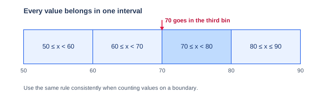
Start the first interval at 50, below the observed minimum of 52, and end the last at 90, above the maximum of 86. For this example, each interval includes its left boundary and excludes its right boundary; the final interval includes 90 if a score of 90 is present:
- 50 ≤ score < 60
- 60 ≤ score < 70
- 70 ≤ score < 80
- 80 ≤ score ≤ 90 (final bin)
Where does 70 go? It belongs to 70 to under 80, not 60 to under 70. Writing the classes merely as “60–70” and “70–80” is ambiguous unless you also state the edge rule. Each usable score must have one and only one home.
Step 5: Make a Frequency Table
Read the list once and place each score in its interval. The frequency table is also the most reliable way to check a hand-drawn result.
Frequency table for 18 test scores
| Score interval | Observed scores | Frequency | Relative frequency |
|---|---|---|---|
| 50 to under 60 | 52, 55, 57, 58 | 4 | 4/18 = 22.22% |
| 60 to under 70 | 61, 62, 63, 64, 66, 68 | 6 | 6/18 = 33.33% |
| 70 to under 80 | 70, 71, 72, 74, 77, 79 | 6 | 6/18 = 33.33% |
| 80 through 90 | 82, 86 | 2 | 2/18 = 11.11% |
| Total | 18 observed scores | 18 | 100% before rounding |
Check 4 + 6 + 6 + 2 = 18, the original sample size. If your frequency total is 17 or 19, search for an omitted or double-counted number, often one lying exactly on a boundary.
Step 6: Draw the Numerical Axes and Bars
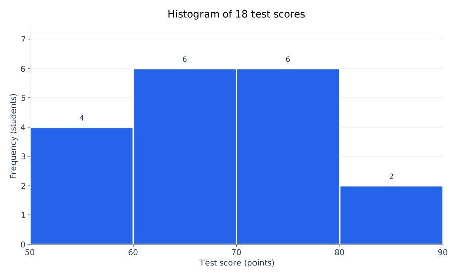
Along the x-axis, mark 50, 60, 70, 80 and 90 at equal ten-point distances. Label it Test score (points). On the y-axis, mark a count scale from zero through at least six and label it Frequency (students). Draw adjacent rectangles spanning 50–60, 60–70, 70–80 and 80–90, with heights 4, 6, 6 and 2.
Do not draw four equal-width decorative category bars disconnected from their numerical boundaries. These happen to have the same width because our intervals all cover ten points. With unequal widths, the rectangle widths must change too, and the appropriate area-based height calculation matters.
Step 7: Label and Check the Finished Histogram
Give the chart a name such as “Distribution of 18 test scores.” Check that the horizontal cutoffs are 50, 60, 70, 80 and 90, that 70 is assigned to the third bin, and that no interval is missing. Confirm the vertical axis says frequency rather than percentage. The finished graph should have no artificial gaps between its consecutive intervals.
Complete Histogram Example: What the Finished Bars Mean
The first bar contains four scores below 60; the second contains six scores from 60 to under 70; the third contains six scores from 70 to under 80; and the fourth contains two scores of 80 or above. The two middle intervals together contain 12/18 = 66.67% of the observations. This is a description of a small class, not evidence of an underlying normal distribution.
The tallest bars are tied. They identify two most-populated intervals under the selected binning, not necessarily two modes in the exact raw scores. All 18 scores in this particular example are distinct, so no score repeats. Read more about the difference between mean, median and mode if you are reporting the numerical center as well as the histogram.
The graph cannot tell you the exact value of each score after the raw list is hidden. It also cannot establish that an unusual observation is a data error. Those questions require inspecting the underlying records.
How to Make a Histogram by Hand
When drawing a histogram on graph paper, begin with the frequency table rather than sketching rectangles by eye. Draw a horizontal number line from 50 to 90, with ten points occupying the same physical distance in every interval. Mark a vertical frequency scale up to six, preferably starting at zero. For each bin, measure its actual width along the x-axis and raise a rectangle to the frequency in the table.
For our example, a rectangle from 50 to 60 rises to four; 60 to 70 rises to six; 70 to 80 also rises to six; and 80 to 90 rises to two. Outline the adjoining bars clearly, but do not put category-style spaces between consecutive intervals. Write “Test score (points)” below the number line and “Frequency (students)” beside the vertical axis. You now have a frequency histogram that can be checked without a computer.
If you have to draw it in an examination, write the interval convention next to your table. A single score such as 70 can otherwise be counted twice or left out when you draw the bars.
How to Make a Histogram From a Frequency Table
Sometimes an exercise supplies the intervals and their frequencies, but not the original measurements. You do not need to invent raw data. Verify that the classes are numerical, ordered, exhaustive and non-overlapping; place their real boundaries on the horizontal axis; then use the supplied counts to draw the rectangles. For equal-width intervals, the bar heights can be the frequencies.
For example, if a table gives 50–<60: 4, 60–<70: 6, 70–<80: 6 and 80–90: 2, the same four-bin histogram can be drawn directly from the summary. What you cannot recover from that table is which exact scores occurred inside each range, or the exact ungrouped mean.
Unequal intervals need an extra step. If one bin spans 20 units and another spans 10, bars of height equal to raw counts make the rectangle areas misleading. Use a frequency-density scale when area is intended to represent counts, or probability density when area is intended to represent proportions. The worked density example below shows why.
How to Make a Relative Frequency Histogram
A relative frequency histogram uses the share of observations in each bin rather than the raw count. Keep the same boundaries and divide each frequency by the number of observations:
Relative frequency = bin frequency ÷ total observations.
For the interval 60 to under 70, that is 6 ÷ 18 = 0.3333, or 33.33%. The other bars represent 4 ÷ 18 = 22.22%, 6 ÷ 18 = 33.33%, and 2 ÷ 18 = 11.11%. The exact fractions add to one; displayed percentages can differ slightly from 100 because of rounding.
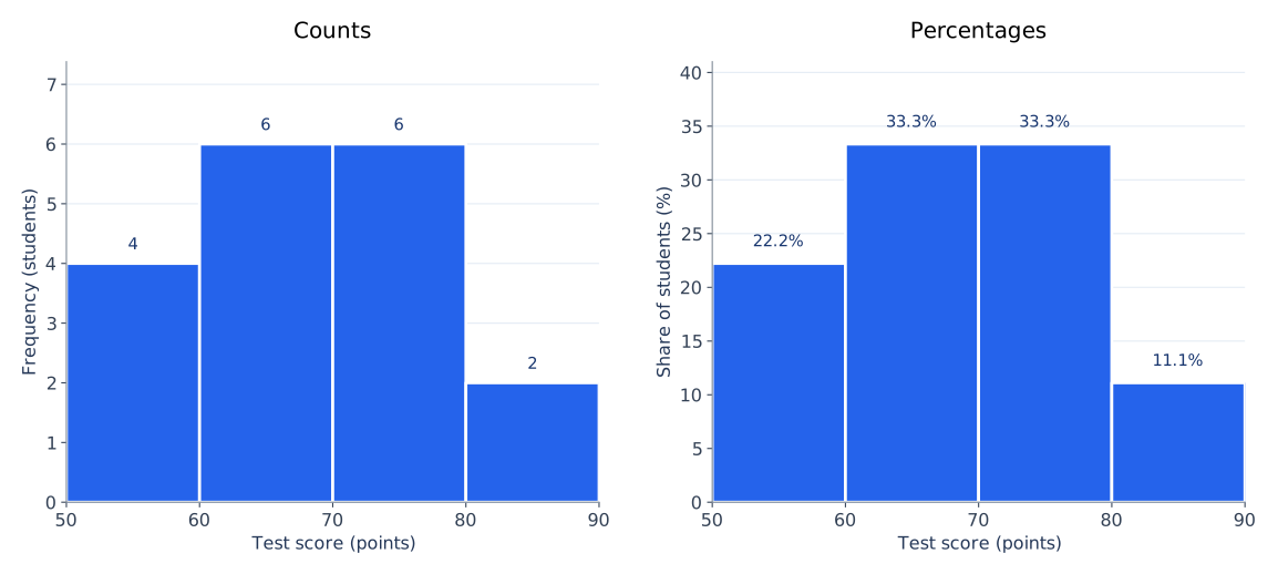
A percentage histogram can be easier to compare with a larger or smaller sample, provided the bin boundaries are comparable. A percentage is not a probability-density height unless it has also been divided by bin width. Likewise, a cumulative frequency chart or an ogive answers a different question: how much of the data lies at or below successive cutoffs.
How to Choose Histogram Bins and Bin Width
Bin settings determine what detail a histogram shows. Two very wide intervals could hide an empty middle region; dozens of narrow intervals could turn ordinary sampling variation into a jagged-looking chart. Neither extreme is automatically more honest. Start with a rule of thumb, then compare a few sensible choices that suit the measurement scale.
Common starting points for bin selection
| Method | Rule | What to remember |
|---|---|---|
| Square-root | k ≈ √n | For n = 18, about 4.24 bins; four is a practical example, though software may round up to five. |
| Sturges | k = ⌈1 + log₂(n)⌉ | For n = 18, six bins. A starting suggestion, not the correct answer for all data. |
| Freedman–Diaconis | width = 2 × IQR × n−1/3 | Uses the middle-half spread; software still has to choose useful edges. |
| Scott | width ≈ 3.5 × standard deviation × n−1/3 | Uses standard deviation; suitable assumptions and sample size matter. |
Here, k is the suggested bin count, n is the number of observations and IQR is the interquartile range. The formulas choose a starting width or count, not the first left boundary. A width of ten beginning at 50 does not group the data the same way as a width of ten beginning at 52.
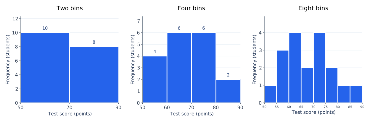
A practical check: if changing from four to five or six bins completely changes your description of the distribution, report that sensitivity. Avoid cherry-picking settings merely because they make the data look more symmetric or more dramatic.
What if Histogram Bins Have Unequal Widths?
Equal-width bins let ordinary frequency serve as bar height without confusing area comparisons. With unequal widths, a 20-point-wide rectangle naturally covers more of the numerical axis than a 10-point-wide rectangle. If area is meant to represent count, use frequency density = frequency ÷ bin width; if area is meant to represent proportion, use probability density = frequency ÷ (n × bin width).
Combine our two middle intervals into one 60-to-under-80 bin. The three new bins are 50–<60 (frequency 4, width 10), 60–<80 (frequency 12, width 20) and 80–90 (frequency 2, width 10). Their frequency-density heights are 0.4, 0.6 and 0.2 counts per score point. Their areas are 4, 12 and 2. Had we drawn the middle height as 12, the much wider bar would exaggerate its frequency when areas are compared.
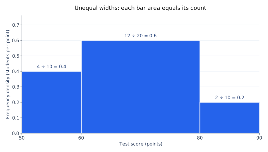
The AmriData maker currently uses equal-width bins and offers count or percentage, not custom unequal-width density bins. For a density chart with exact edges, use a charting workflow that explicitly supports the intended widths and scaling.
How to Make a Histogram With AmriData
Open the Histogram Maker if you want to graph numbers without drawing the bins or setting up a spreadsheet. Its current free tool processes pasted values in browser JavaScript and lets you choose automatic (Sturges), square-root or custom bin counts, plus a count or percentage y-axis.
- Open AmriData Histogram Maker.
- Paste the same 18 scores into the Your data field, separated by commas or new lines.
- Choose Auto (Sturges) for an automatic starting count; or choose √n or Custom and enter a count.
- Under Y-axis, select frequency (count) or relative frequency (%).
- Optionally set a chart title, bar color and mean or median reference lines.
- Click Generate Histogram and check the count, minimum, maximum and plot.
- If the output looks useful, select Download PNG to save the image.
Why won't custom four bins look exactly like the hand example? The current maker allows you to select the number of equal-width bins but does not expose independent fields for starting edge 50, ending edge 90 or fixed width 10. It generally uses the observed data span (52 to 86) to form equal-width intervals. Custom “4” therefore does not mean “50–60, 60–70, 70–80, 80–90.” Both results can be valid; compare their actual boundaries before comparing their frequencies.
The privacy statement above applies to this standalone browser tool, not automatically to file uploads or every other AmriData service. The current online controls should be rechecked when this tutorial is updated.
How to Make a Histogram in Excel
In modern desktop Microsoft Excel, the quickest route uses its built-in statistical histogram chart. Put the observations in a single column; do not replace them with the four summarized frequencies for this workflow. Here is how to make a histogram in Excel using the 18 scores:
- In cell A1, type Score. Enter the 18 numbers in A2:A19, one number in each cell.
- Select the numeric cells, optionally including the column heading.
- Go to Insert → Insert Statistic Chart → Histogram. In some Excel versions or ribbon layouts, the command is under Statistical.
- Select or right-click the horizontal axis, choose Format Axis, and open Axis Options.
- Choose Bin width and enter 10, or choose a Number of bins. Compare the result with the automatic setting.
- Inspect any Underflow bin or Overflow bin options only if you need to combine scores below or above a threshold.
- Give the chart an informative title and check its frequency axis and displayed bin boundaries.
Excel's bin-edge detail matters: entering width 10 does not, by itself, guarantee the exact starting boundary 50 used in our hand example. If the displayed bins begin elsewhere, the frequencies can differ even though the 18 raw scores are identical. Do not claim a match to 4–6–6–2 until you check the actual interval labels. Excel's automatic chart binning may use a Scott-type reference rule, and the exact menus vary across Excel versions and Mac.
How to check exact 50–60–70–80–90 classes in Excel
When your assignment requires those exact limits, you can build a separate frequency table with formulas. If the raw numbers occupy A2:A19, these formulas use the same left-inclusive, right-exclusive rule as the hand example:
=COUNTIFS($A$2:$A$19,">=50",$A$2:$A$19,"<60")
=COUNTIFS($A$2:$A$19,">=60",$A$2:$A$19,"<70")
=COUNTIFS($A$2:$A$19,">=70",$A$2:$A$19,"<80")
=COUNTIFS($A$2:$A$19,">=80",$A$2:$A$19,"<=90")
The formulas return 4, 6, 6 and 2. They verify the custom table; they do not force Excel's built-in histogram chart to use these edges. If you chart these summarized frequencies with ordinary columns, label and scale the numeric intervals correctly and avoid presenting a category column chart as if it automatically preserved unequal numerical widths. The older Data → Data Analysis → Histogram route is an optional Analysis ToolPak method with its own bin-end conventions, not the same menu as Insert Statistic Chart.
How to Make a Histogram in Google Sheets
Google Sheets calls histogram intervals buckets in its chart editor. Use raw numerical observations in one column, just as you did in Excel.
- Open a sheet. Enter Score in A1 and paste the 18 values into A2:A19.
- Select the data and choose Insert → Chart.
- In the Chart editor's Setup section, choose Histogram chart under chart type.
- Open Customize → Histogram and look for Bucket size.
- Try a bucket size of 10, then inspect where the bucket boundaries begin and end.
- Use Customize → Chart & axis titles to label the score variable and the frequency axis. Other available options include item dividers and outlier percentile.
- Confirm the number of observations represented and adjust the bucket setting if the chart hides too much detail.
“Bucket size 10” sets an interval width, not necessarily the exact origin of the hand-drawn bins. Different automatic boundaries may change the counts. Check the horizontal axis before claiming that Sheets reproduces the four-bin frequency table.
If your assignment is being written in Google Docs, create the histogram in Google Sheets first and then insert or copy the chart into Docs. Google Docs does not use the same histogram chart editor that Sheets does.
How to Make a Histogram in Python With pandas
For data already stored in a Python data-analysis workflow, pandas offers a short route. Its DataFrame.hist() method uses Matplotlib for rendering by default; it is a convenient wrapper, not a separate statistical definition of a histogram. Install pandas and Matplotlib in your Python environment if they are not already available.
The following code uses the same four explicit bin edges as the hand calculation, so the histogram should have heights 4, 6, 6 and 2:
import pandas as pd
import matplotlib.pyplot as plt

scores = [52, 55, 57, 58, 61, 62, 63, 64, 66,
          68, 70, 71, 72, 74, 77, 79, 82, 86]

df = pd.DataFrame({"Score": scores})
ax = df.hist(column="Score", bins=[50, 60, 70, 80, 90],
             edgecolor="white", grid=False)[0, 0]
ax.set_title("Distribution of 18 test scores")
ax.set_xlabel("Test score (points)")
ax.set_ylabel("Frequency (students)")
ax.set_xticks([50, 60, 70, 80, 90])
plt.tight_layout()
plt.show()
Using bins=4 instead asks the plotting function to calculate four intervals from the data, which generally will not be anchored at 50. Using bins=[50, 60, 70, 80, 90] locks the precise edges. If you have a DataFrame with several numerical columns, DataFrame.hist() can produce separate charts, but start with one variable when verifying the example.
How to Make a Histogram With Matplotlib
Matplotlib's direct pyplot.hist() function is useful when you want explicit control over the bins, axes and figure. Unlike the pandas example, you pass the list of observations straight to the plotting function. This also makes the bin setting visible at the point where the histogram is drawn.
import matplotlib.pyplot as plt

scores = [52, 55, 57, 58, 61, 62, 63, 64, 66,
          68, 70, 71, 72, 74, 77, 79, 82, 86]

counts, edges, patches = plt.hist(
    scores,
    bins=[50, 60, 70, 80, 90],
    edgecolor="white"
)
plt.xticks([50, 60, 70, 80, 90])
plt.xlabel("Test score (points)")
plt.ylabel("Frequency (students)")
plt.title("Distribution of 18 test scores")
print("Bin counts:", counts.astype(int).tolist())
plt.tight_layout()
plt.show()
The printed counts should be [4, 6, 6, 2]. Both pandas and Matplotlib follow numerical bin boundaries; with this explicit edge sequence, a value equal to 70 belongs to the 70–<80 bin, while the last right-hand endpoint is included. Matplotlib also accepts an integer bin count or supported automatic selection strings, but those modes choose different boundaries.
If you start from a frequency table rather than raw scores, you cannot reconstruct the missing individual observations just to call hist(). Plot the known intervals and heights with appropriate numerical widths, or calculate the area-correct heights for unequal bins.
Which Histogram-Making Method Should You Use?
Every method above can produce a legitimate histogram, but its default control and the work required are different. If you need an exact hand-graded four-bin chart, explicit boundaries are usually more important than which program you choose.
Methods at a glance
| Method | Best suited to | How to set bins | Important limitation |
|---|---|---|---|
| By hand | Learning and classroom work | Draw exact edges yourself | Slow for large samples |
| AmriData | Fast online histogram and PNG | Automatic, √n or custom count | No independent exact-edge controls currently |
| Excel | Spreadsheet reports | Automatic, bin width or count in Format Axis | Check chart's actual origin and version |
| Google Sheets | Collaborative spreadsheets | Bucket size in chart editor | Bucket origin may differ from hand example |
| Python/pandas | DataFrames and repeatable analysis | Explicit edges in df.hist() | Requires Python libraries |
| Matplotlib | Precisely controlled figures | Explicit edges in plt.hist() | Requires a little plotting code |
Why Do Excel, Sheets, AmriData and Python Show Different Histograms?
First compare the data. Is the same set of 18 numeric observations in every program, with blanks and text handled consistently? Then compare the number of bins, starting edge, ending edge and interval width. A chart that starts at 52 with four equal-width bins across 52–86 is different from one anchored at 50 with four ten-point bins through 90.
Automatic bin rules also vary. Excel documents a Scott-type automatic method for its built-in histogram chart; the current AmriData default is Sturges; pandas and Matplotlib follow the settings passed to their plotting functions. There is no contradiction when each program assigns the same raw values to different intervals. To make a fair comparison, configure identical cutoffs where supported, then compare the resulting counts.
A subtle difference can also arise from where a boundary value goes. Explicitly defining [60,70) and [70,80) puts 70 in the third class. A tool or legacy workflow that treats right ends as inclusive might assign it differently. Read its interval labels and documented counting rule rather than assuming every histogram command uses identical endpoint conventions.
Histogram vs Bar Chart: Which Graph Are You Making?
A histogram groups a numerical variable into ranges. Its horizontal positions and, when widths vary, rectangle widths represent real numeric distances. A bar chart compares named groups, such as subjects, colors or departments. The category order can often be changed without altering the meaning. Histograms are usually drawn with adjoining interval bars; bar charts usually leave gaps, but touching bars alone are not a complete definition.
If you are graphing “Math, Science and History” as three categories, choose the Bar Chart Maker. If you are graphing the individual scores of students in Math, use a histogram. The full histogram vs bar graph comparison explains the distinction with examples, and AmriData's guide to choosing a chart type helps with other cases.
If you want a compact summary of quartiles, spread and possible extreme values instead of counts in bins, a box plot may be more useful. You can also learn how to make a box plot using the same hands-on approach.
Common Mistakes When Making a Histogram
- Using category labels as bins. Colors and product names are not numerical intervals; use a category bar chart.
- Overlapping classes. “60–70” followed by “70–80” is ambiguous without a boundary rule; write 60 ≤ x < 70 and 70 ≤ x < 80.
- Failing the count check. Frequencies that do not sum to n usually indicate a missing observation or double-counted boundary value.
- Drawing gaps between consecutive intervals. This can make the display look categorical; preserve the x-axis's numeric continuity.
- Assuming bars touching makes any graph a histogram. The underlying numerical intervals are what matter.
- Treating automatic bins as the only correct choice. Compare reasonable widths and starting edges.
- Leaving the vertical axis unlabeled. A height of six could represent six observations, 6% or density; state which one.
- Using raw count as height for unequal widths. If area encodes count, divide by width instead.
- Calling a roughly bell-shaped sample “normally distributed.” A histogram is a visual check, not a proof of a probability model.
- Calling an isolated bar an outlier test. Inspect the raw values before drawing conclusions.
- Expecting different programs to match by default. Their bin algorithms and starting positions may differ.
- Using Excel's ordinary column chart for raw values. A frequency chart with category labels is not automatically a properly scaled histogram.
- Counting blanks as zero or mixing units. Either mistake changes the distribution before any chart is drawn.
- Comparing histograms with different cutoffs as though their bars match. Align the x-axis and bins first.
For broader chart checks, including scales and overdecorated graphics, see common data visualization mistakes. A histogram is most useful when it reflects the measurements rather than a preferred story.
Troubleshooting a Histogram That Looks Wrong
Why do my frequencies add up to only 17?
Compare every observation against your intervals. Look especially for 70 or another score equal to a boundary, a hidden blank, a value stored as text, or a final interval that fails to cover the maximum. Each usable observation should be counted exactly once.
Why did the software create more bars than I expected?
An automatic option may choose six or more intervals rather than the four in the example. Switch to a custom bin count or width where available, then check the starting edge. Bin count and bin origin are separate decisions.
Why does my histogram look more skewed after I change bins?
Moving boundaries may shift values between bars and expose or hide apparent peaks. Recheck the data, then compare multiple sensible settings. Do not infer a permanent distribution shape from one fragile arrangement of bins.
Should I use a histogram for five observations?
You can, but a dot plot or a simple list may show the observations more clearly. A handful of values rarely supports a reliable claim about the shape of a population distribution.
Practice: Construct Your Own Histogram
Try these ten values without looking ahead: 12, 14, 15, 17, 18, 21, 22, 24, 26, 29. Choose four left-inclusive intervals 10–<15, 15–<20, 20–<25 and 25–30 (including 30 in the final class), then count each observation.
Answer: the bin counts are 2, 3, 3, 2, totaling ten. The percentages are 20%, 30%, 30%, 20%. If you assigned 15 to the first bin, the first count would be incorrect under the stated rule. This is a quick way to test whether your frequency table and chart agree.
Once the counting becomes routine, use the same checks as part of an exploratory data analysis workflow: look for unexpected ranges, missing entries and potentially interesting groupings before interpreting the result.
Frequently Asked Questions About Making Histograms
How do you make a histogram step by step?
To make a histogram, collect numerical observations, find their minimum and maximum, choose non-overlapping bins, count observations per bin, draw the rectangles over a numerical x-axis, and label the axes. With equal-width bins, the rectangle heights can show the counts directly.
What type of data do you need for a histogram?
Use numerical data such as scores, heights, amounts or waiting times. Both measurements and suitable discrete numerical observations can work. Categories such as colors or departments call for a bar chart instead.
How many bins should a histogram have?
There is no universal number. Start with a rule such as √n or Sturges, then adjust for sample size, measurement resolution, audience and the question you want to answer. Our 18-score example uses four bins for clarity; Sturges suggests six.
How do you calculate bin width?
Divide the observed range by the number of bins as a starting estimate. For 18 scores ranging from 52 to 86, 34 ÷ 4 = 8.5. We choose width 10 and edges from 50 to 90 for an easy-to-read manual chart.
Can you make a histogram from a frequency table?
Yes. Put the class boundaries on a scaled x-axis and use the supplied frequencies for equal-width bars. With unequal widths, use frequency density if areas are meant to encode counts. You do not need to invent raw data.
How do you make a relative frequency histogram?
Divide each frequency by the total number of observations and keep the same bins. For six scores out of eighteen, the relative frequency is 6/18 = 0.3333, or 33.33%.
Which bin contains a value that falls exactly on the boundary?
State the convention. In this guide, bins include their left edge but exclude their right edge, except for the final interval. A score of 70 therefore goes into 70–<80, not 60–<70.
How do you make a histogram in Excel?
Enter the observations into a column, select the cells, and choose Insert → Insert Statistic Chart → Histogram in modern Excel. Use the horizontal-axis Format Axis panel to adjust bin width or count, and check the displayed edges.
How do you change histogram bins in Excel?
Select the chart's horizontal axis, choose Format Axis, and find the Bin width or Number of bins settings. Underflow and overflow bin options are also available for some chart configurations. A chosen width alone does not guarantee a chosen first edge.
How do you make a histogram in Google Sheets?
Put numeric observations in a column, choose Insert → Chart, select Histogram chart as the chart type, then adjust Customize → Histogram → Bucket size if needed. Add descriptive chart and axis titles.
How do you create a histogram in Python?
With pandas, call DataFrame.hist() on a numeric column and pass a bin count or exact edges. For greater control, use matplotlib.pyplot.hist(data, bins=[...]) directly and set the axis labels and title.
Do histogram bars have to touch?
Bars over consecutive intervals are generally adjacent because the x-axis is a continuous numerical scale. The real distinction from a category bar chart is the meaning of the numerical intervals, not merely the presence or absence of a visible gap.
Can a histogram have unequal bin widths?
Yes. Draw bars at their true numerical widths, and use an area-correct height such as frequency density (frequency divided by width) when area represents count.
Why do two programs produce different histograms of the same data?
They may use different automatic bin counts, widths, starting edges or boundary rules. Match the raw data and explicit interval cutoffs before deciding whether the results genuinely disagree.
Key Takeaways
- Start with one numerical variable, inspect its range and define bins that cover every usable observation exactly once.
- For the 18-score example, edges 50, 60, 70, 80 and 90 give frequencies 4, 6, 6 and 2.
- With equal-width bins, height can show frequency or percentage; with unequal widths, use an area-correct density when appropriate.
- Automatic software bins are starting suggestions, not universally correct settings. Compare explicit boundaries before comparing software output.
- Keep the numerical scale, bin convention, sample size and vertical units clear for the reader.
Knowing how to make a histogram means being able to explain each rectangle, not only generating a chart. Try the Histogram Maker to plot your own values, or return to the Data Visualization category for other step-by-step chart guides.
Related Data Visualization Guides and Tools
- Data Visualization guides — return to the main category for chart-making tutorials
- Histogram Maker — paste raw numbers and export a histogram as PNG
- What Is a Histogram? — learn the definitions, types and how to interpret a histogram
- Histogram vs Bar Graph — see which chart fits numerical intervals versus categories
- How to Choose the Right Chart Type — match a visual to your analytical question
- How to Make a Box Plot — another hands-on guide for quantitative data
- Exploratory Data Analysis Steps — use histograms in a practical analysis process
← Back to all Data Visualization articles
References and Software Documentation
- NIST/SEMATECH e-Handbook — Histogram. Background on histogram construction and distribution analysis.
- Microsoft Support — Create a Histogram. Modern Excel chart commands and Format Axis options.
- Google Docs Editors Help — Histogram Charts. Sheets data format and bucket-size controls.
- pandas documentation — DataFrame.hist. Histogram method and Matplotlib backend.
- Matplotlib documentation — pyplot.hist. Bin edges and direct charting.
- AmriData Histogram Maker. Current online tool controls and processing statement.