
Histogram shapes (often searched as the types of histogram distributions) describe the pattern made by bars across a numerical range. The common shape names are symmetric, bell-shaped (mound-shaped), uniform, right-skewed, left-skewed, unimodal, bimodal and multimodal. Less common names include J-shaped and U-shaped. To name a shape, look at the balance of the two sides, the direction of the longer tail and the number of apparent peaks. One histogram can have more than one of these descriptions.
A shape is a clue, not a diagnosis. The same data can look different with a new bin width, and even a neat bell-shaped histogram cannot prove that its population follows a normal distribution. Below, the pictures are drawn from documented, reproducible synthetic samples rather than arbitrary bar heights. Quality-control names such as plateau, comb, edge peak, truncated and dog food are covered in their own section.
This guide belongs to AmriData's Statistics category. For bin definitions, see what a histogram is; to construct a chart from values, use how to make a histogram.
Types of Histogram Shapes and What They Mean
Start with these six pictures. They show different distributions, each simulated with 1,200 observations. The bars are sample frequencies, so small bumps and dips are normal.
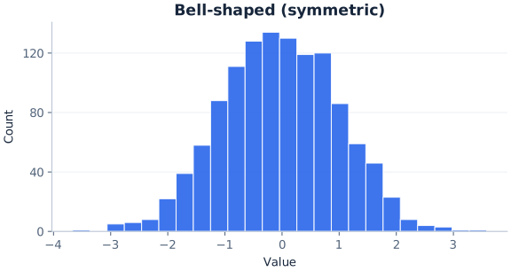


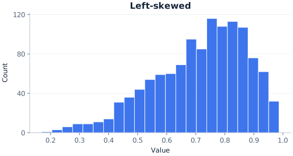
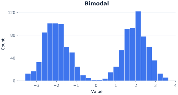

The quick pictures are separate examples; their horizontal scales measure different variables or distribution units. The shapes can be compared visually, but their x-axis numbers should not be treated as directly comparable measurements.
Histogram shape names, visual clues and what they may mean
| Shape | Visual clue | What it may mean | What to check |
|---|---|---|---|
| Symmetric | Overall structure balances around the middle | Values spread in a similar way on both sides of a central location | Does the balance persist with nearby bin settings? |
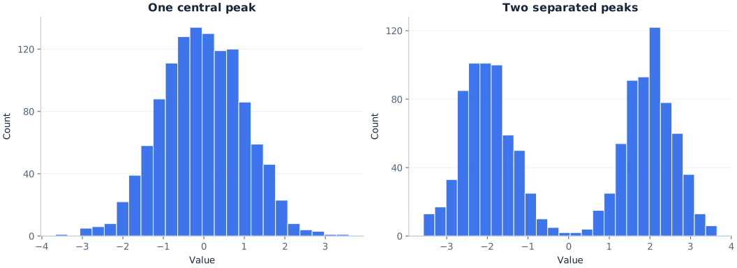
| Bell-shaped (mound-shaped) | One central peak; frequencies decline toward either end | Most values sit near a typical level; extremes are less common | A bell-like appearance is not proof of normality |
| Uniform-like | No strong peak; broadly similar bar heights | Values occur at similar rates across the range, or the bins are too wide to show a peak | Uneven bars may be ordinary sampling variation; try more bins |
| Right-skewed | Longer tail toward higher numerical values | Most values are modest and a few are much larger, often above a floor such as zero | Follow the tail, not the tallest bar |
| Left-skewed | Longer tail toward lower numerical values | Most values are high and a few are much lower, often below a ceiling such as 100 | Follow the tail, not the tallest bar |
| Unimodal | One main peak | A single concentration of values | The highest bin is not necessarily the raw-data mode |
| Bimodal | Two apparent peaks | Possibly two groups, shifts, machines or conditions mixed together | Check bin sensitivity and split the data by group |
| Multimodal | Three or more apparent peaks | Several groups, or noise from small samples or narrow bins | Rule out noise or grouping artifacts before explaining them |
| J-shaped / reverse J | Frequencies climb (or fall) steadily to one edge | An extreme skew, often next to a hard limit | Check whether a boundary or screening creates the edge |
| U-shaped | Tall bars at both ends, low middle | Values gather at two extremes | Check scale limits and whether two groups are present |
| No clear pattern (erratic) | Ragged bars with no stable outline | Often too many bins or too few observations | Try fewer bins or collect more data |
Histogram Shapes vs Types of Histograms
When people search for “types of histograms,” they usually mean the shape names above. The phrase can also refer to different ways of drawing the chart: a frequency histogram (bar height is a count), a relative frequency histogram (bar height is a proportion or percentage), a density histogram (bar area is a proportion) and a cumulative histogram (each bar is a running total). Those are chart types, not shapes.
With equal-width bins, frequency, relative frequency and density histograms of the same data have the same shape; only the vertical scale changes. A cumulative histogram always rises from left to right, so the shape names in this guide do not apply to it in the same way.
How to Describe the Shape of a Histogram
A useful description has three layers. First, decide whether the bulk of the observations is roughly balanced around the middle or has a longer tail on one side. Next, count clear peaks. Finally, note gaps, clusters, unusually sparse outer ranges and whether the impression changes under sensible bin choices.
Many statistics courses place shape inside a wider checklist: describe the shape, the center, the spread and any unusual features such as gaps or possible outliers. Shape comes first because it affects which center and spread are sensible to report. For a strongly skewed sample, the median and interquartile range often summarize the data better than the mean and standard deviation.
- Check the horizontal axis. It should show numerical intervals. A chart of colors or departments needs a bar chart, not a histogram.
- Look for symmetry or skew. Compare the general mass and tail lengths, not individual matching bars.
- Count main peaks (the modality). One means unimodal; two suggests bimodal; three is sometimes called trimodal; more than two is multimodal. No clear peak suggests a uniform-like shape.
- Inspect the edges. A long sparse tail can matter even when its bars are short.
- Look for interruptions. An empty bin may reflect a meaningful gap or simply one choice of boundaries.
- Test another sensible grouping. Persistent patterns are more convincing than a feature that disappears immediately.
For example, “approximately symmetric and bimodal, with a low-frequency gap between the two peaks” tells a reader considerably more than “symmetric.” Likewise, “unimodal and right-skewed” combines a statement about peaks with one about asymmetry, and “roughly uniform between 0 and 1, with no clear peak” describes both the outline and the range. These names are not mutually exclusive categories.
Symmetric Histogram
A symmetric histogram has a broadly similar pattern on either side of its center. Imagine folding the distribution around its middle: the two halves would have comparable overall weight and shape, though their individual bins need not match. Symmetrical histogram and symmetric histogram are two names for the same idea.
Symmetry says nothing by itself about the number of peaks. A bell-shaped distribution may be symmetric, but so may a roughly uniform distribution or one with two equally placed peaks. In fact, the three examples below have different patterns even though each is approximately symmetric in its underlying model.
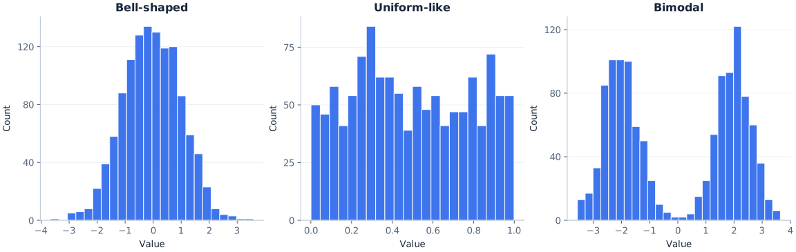
Symmetric histogram examples: the totals from rolling two dice many times (a triangle-like shape that peaks at 7), repeated measurements of one object with a well-calibrated instrument, and heights in a large sample of adults of one sex often look roughly symmetric. None of these is guaranteed to; the sample, the bins and the way the data were collected still matter.
What it may suggest: the sample distribution is fairly balanced around a central location. Do not assume: the underlying population must be normal or that the sample mean and median are exactly equal. With real data, the symmetry judgment is approximate.
Symmetric vs Uniform vs Bell-Shaped Histograms
These three names overlap, which is why they are easy to mix up. Symmetric is a property: the two sides balance. Uniform and bell-shaped describe the outline. A uniform-like histogram is usually also roughly symmetric, and so is a bell-shaped one, but a symmetric histogram need not be either. A symmetric bimodal or U-shaped histogram is neither flat nor bell-like.
How symmetric shapes differ
| Description | Peaks | Outline | Example wording |
|---|---|---|---|
| Symmetric and bell-shaped | One, in the middle | Tall center, tapering sides | “approximately symmetric and bell-shaped” |
| Symmetric and uniform | No clear peak | Broadly flat across the range | “roughly uniform, and so roughly symmetric” |
| Symmetric and bimodal | Two, balanced | Two mounds with a dip between them | “symmetric and bimodal” |
| Symmetric and U-shaped | Two, at the edges | High ends, low middle | “U-shaped and roughly symmetric” |
When a textbook question asks which histogram is “approximately uniform,” look for the chart whose bars stay at broadly similar heights with no sustained mound. Small differences between neighboring bars do not rule it out. When it asks which histograms are “approximately symmetric,” a uniform-like chart, a bell-shaped chart and a balanced two-peaked chart can all qualify.
Bell-Shaped Histogram
A bell-shaped histogram has one prominent central mound. Moving from the center toward either end, frequencies tend to decline. A classic normal distribution has this general population shape, but a real histogram is a set of bars drawn from a finite sample. Random samples almost always contain local irregularities.
Use “approximately bell-shaped” when a sample has a clear central concentration, tapering tails and roughly balanced sides. Do not insist on a perfectly smooth outline. A bell-shaped histogram is usually also described as unimodal and approximately symmetric, because those labels describe different properties. Some textbooks say mound-shaped for the same idea; it is a slightly looser word that does not suggest any particular mathematical curve.
What it may suggest: a single central region where observations are common, with fewer observations toward the extremes. Repeated measurement errors and many physical measurements from a stable process often look like this. Do not assume: the chart demonstrates a specific distribution family, an absence of outliers, or exact normality.
Is a Bell-Shaped Histogram Normal?
Not necessarily. “Bell-shaped” is a visual description; “normal distribution” is a specific mathematical probability model. A normal density has a smooth theoretical curve determined by its mean and standard deviation. A histogram shows observed counts or densities in bins. They are not the same object.
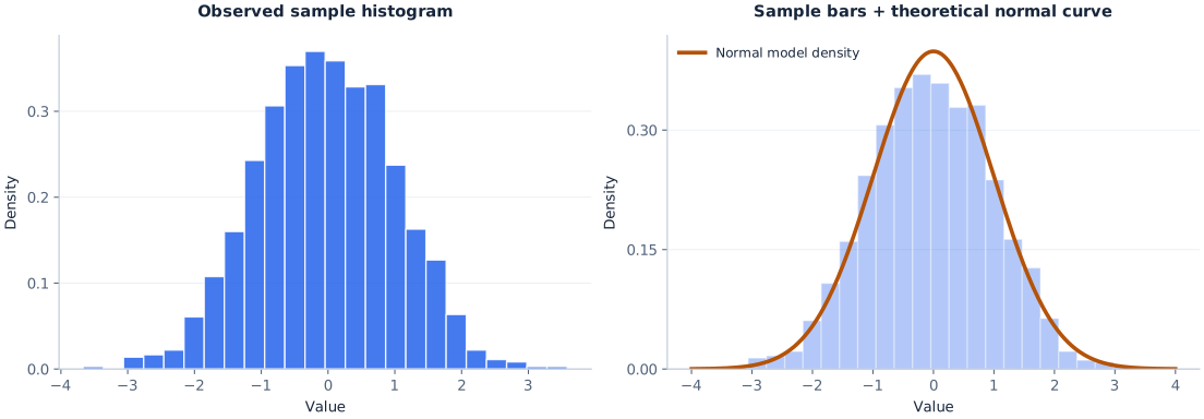
An approximately normal histogram often looks bell-shaped, and it may be reasonable to describe a sample as “normal-like.” That still does not establish a normal population. A different symmetric unimodal distribution could have a similar display; small samples and different bins can be misleading. Where normality is a substantive assumption, inspect a Q–Q plot, the study context and any appropriate additional diagnostics. The main histogram guide covers related chart basics without treating shape as a formal distribution test.
Uniform Histogram
A uniform histogram looks relatively flat: no part of its range stands out as a large, sustained peak. If a variable is uniformly distributed over an interval, equal-width intervals are equally likely in the population. But a random sample from that population does not put exactly the same number of observations into each bin.
The example in the opening grid uses simulated Uniform(0,1) values. Its bar heights vary, yet the overall pattern lacks a pronounced mound. That is why “approximately uniform” or “uniform-like” is better than demanding a row of identical rectangles.
Uniform histogram examples: many rolls of a fair die, draws from a computer's random-number generator and lottery numbers tend to produce roughly flat charts. A flat look can also come from how the chart was built rather than from the data. Very few, very wide bins can average a peak away, and pooling several sources with different centers can fill in the dips between their mounds. Before calling data uniform, try more bins and split the data by source.
What it may suggest: observations occur at relatively similar rates across the displayed range. Do not assume: the generating process is truly uniform, or that any unequal bar heights disprove uniformity. A roughly flat histogram can also be approximately symmetric, which makes it quite different from a bell shape despite sharing that symmetry property.
Right-Skewed Histogram (Positively Skewed)
A right-skewed histogram has a relatively long or thin tail extending toward larger numerical values. Much of the data may sit on the lower end, while a smaller number of observations stretch the display far to the right. Positive skew and skewed right refer to this same direction.
Right skew often appears when values have a natural floor. Waiting times, prices, transaction amounts and insurance claims cannot fall below zero, but a few can be very large, so the data bunch up near the floor and trail off to the right. These variables are not guaranteed to be skewed in every study. In process data, skew caused by a physical limit can be the usual, expected pattern rather than a sign of trouble. In the synthetic example, an exponential distribution provides a clear right tail.
Left-Skewed Histogram (Negatively Skewed)
A left-skewed histogram has a longer tail extending toward smaller numerical values. The taller bars may instead lie toward the upper end. Imagine an easy exam where many scores are high but a minority of much lower scores extends the distribution leftward; that would be a plausible example, not a rule for all easy exams.
Left skew often appears under a ceiling. Percentage scores cannot go above 100, so when most results are near the top, the only room for the tail is on the left. The illustrated sample uses Beta(5,2) data, which cluster toward larger values on a scale from zero to one. Negative skew and skewed left are equivalent names in this context.

A practical check: if you confuse the two names, ignore the peak for a moment. Look only at which end contains the more extended, thinly populated tail. It is the direction in which values trail off, not the direction in which most values pile up.
Skewed Left vs Skewed Right at a Glance
Comparing the two skew directions
| Right-skewed | Left-skewed | |
|---|---|---|
| Also called | Positively skewed, skewed right | Negatively skewed, skewed left |
| Longer tail points | Toward larger values | Toward smaller values |
| Tallest bars usually sit | Toward the low end | Toward the high end |
| Mean compared with median | Often above the median (not guaranteed) | Often below the median (not guaranteed) |
| Typical cause to check | A floor such as zero | A ceiling such as a maximum score |
Unimodal Histogram
A unimodal histogram has one main apparent peak. The mound may be balanced, such as a bell shape, or noticeably asymmetric, such as a right-skewed mound. “Unimodal” describes the number of peaks; it does not describe symmetry, tail length or a particular mathematical distribution. So yes, a histogram can be unimodal and skewed at the same time.
The most populated bar is the modal bin for the chosen intervals. It identifies a range with the highest frequency, not necessarily the exact most common original value. If the underlying variable is measured continuously, most raw values might not repeat at all. For the distinction between a distribution's mode, mean and median, see the mean, median and mode guide.
Bimodal Histogram
A bimodal histogram (sometimes called double-peaked) has two apparent peaks, often separated by a lower-frequency interval. It may prompt questions about separate groups, measurement conditions or repeated processes. Suppose measurements were taken in two operating modes of a machine: two concentrations might appear. But the chart alone cannot establish that explanation.
The synthetic bimodal example combines 600 values from Normal(−2,0.6) and 600 from Normal(2,0.6). Its two clusters are intentionally generated, not discovered in a real business dataset. With reasonable bins, the higher regions are visible to either side of zero. It is also roughly symmetric as a whole.
In quality work, a bimodal histogram is a standard prompt to stratify: draw separate histograms for each shift, machine, supplier or batch on the same scale, and see whether each one is unimodal on its own.
What it may suggest: two concentrations worth investigating. Do not assume: the sample proves the presence of exactly two populations. A short sample, rounding, uneven data collection, or unusual bin boundaries can create or hide local peaks.
Multimodal Histogram
A multimodal histogram has more than two apparent peaks; one with exactly three is sometimes called trimodal. The opening illustration uses three simulated normal groups centered at different locations. This creates a clear teaching example, but real datasets can show extra bumps for far less interesting reasons: randomness, measurement precision, small numbers of observations, or unsuitable bins.
When a plot looks multimodal, inspect the raw values and any group labels. If measurements come from several machines, shifts, regions or time periods, draw separate histograms on a shared scale before declaring those groups responsible. You can describe a histogram as multimodal and approximately symmetric when both properties apply. When many peaks sit close together, they can merge into a flat-topped plateau.
J-Shaped, Reverse J-Shaped and U-Shaped Histograms
These names describe the outline more literally. They appear in some textbooks and exam questions, and books differ slightly in how they use them, so it is worth saying which end is high rather than relying on the letter alone.


A J-shaped histogram has few observations on the left and frequencies that rise toward the right edge, like the letter J. It is an extreme form of left skew in which the tallest bar sits at, or next to, the top of the range. A reverse J-shaped histogram is the mirror image: the tallest bar is at the low end and frequencies fall away steadily, an extreme form of right skew. Counts in which zero is the most common value, such as the number of support tickets each customer opens in a month, often look like this.
A U-shaped histogram has its tallest bars at both ends and its lowest bars in the middle. It can appear when values gather at two extremes, such as two groups at opposite ends of a scale. It has two peaks, but they sit at the edges of the range rather than inside it. If the variable has only a handful of possible values, such as a five-point rating, a bar chart of each value is usually clearer than a histogram.
The illustrations use Beta(5,1), Beta(1,5) and Beta(0.5,0.5) samples of 1,200 values each.
Histograms With No Clear Shape
Sometimes no single name fits: bars jump up and down without a stable outline. Quality references sometimes call this a random or erratic pattern. It often comes from too many narrow bins, too few observations, or several unrelated sources pooled together. Try fewer bins, check the sample size and split the data by source before concluding that the variable has no structure.
Histogram Patterns in Quality Control: Plateau, Comb, Edge Peak, Truncated and Dog Food
Quality engineers read histograms of process measurements, and the classic quality-tool literature, including ASQ's histogram guidance, gives names to patterns that point to how data were produced, recorded or sorted. Treat each name as a lead to investigate, not a verdict.
One note first: in process work, “normal” often means typical for that process. A process with a natural limit on one side may produce a skewed histogram as its usual, healthy pattern, even though the distribution is not normal in the statistical sense.


Quality-control histogram patterns and what to check
| Pattern | What it looks like | Common explanation to check | Next step |
|---|---|---|---|
| Plateau | Flat top across several bins, sloping sides | Several similar groups with nearby centers blended together | Stratify by machine, operator, batch or time |
| Edge peak | Otherwise smooth shape with an unusually tall bar at one end | Values beyond a cut-off grouped into one “over” or “under” bin, or out-of-range readings recorded at the limit | Read the bin definitions and the raw records |
| Comb | Alternating tall and short bars | Rounding or instrument resolution that does not fit the bin width | Make the bin width a whole multiple of the measurement step |
| Truncated (heart-cut, cliff) | A mound that stops abruptly on one or both sides | Items outside limits removed by inspection before the data were recorded | Ask whether the data were screened; measure before sorting |
| Dog food | Values near both limits but a hole in the middle | The central, best-fitting output sent elsewhere, leaving the remainder | Trace how the product was sorted upstream |
| Isolated peak | A small separate cluster away from the main body | A different source, a setup or measurement error, or genuine rare values | Inspect those records individually |
The comb illustration shows the most common cause. The simulated gauge reports to the nearest 0.2 mm, but the bins are 0.3 mm wide, so some bins can collect two possible readings while their neighbors collect only one. The dog food name comes from the idea that one customer receives the choice central cut and another is left with the odds and ends on either side of it.
A comb or edge peak is usually fixed by rebuilding the chart. A plateau, truncation or dog-food shape is usually a fact about how the data were produced, and it needs a conversation with whoever collected them.
Histograms With Gaps, Clusters and Extreme Regions
A gap is a numerical interval with few or no observed values. A cluster is an area where many observations gather. The low middle region in the bimodal illustration resembles a separation between clusters; the extent of that separation depends on the sample and the bins.
Do not conclude from one empty bar that intermediate measurements are physically impossible. An instrument might round values, a dataset might contain small sample counts, or the interval might simply have received no observations. A gap deserves a look at how the measurements were obtained.
Likewise, a lonely bar far from the main body is a reason to inspect the underlying observations, not proof of a statistical outlier. Read the raw entries, units and context. For a compact way to examine quartiles and potentially unusual points, read how box plots summarize distributions; for formal rules, see how to find outliers.
How Mean and Median Relate to Histogram Shape
Skewed samples often show differences between the mean and median. In many right-skewed distributions, a small number of high values pulls the mean above the median. In many left-skewed distributions, lower tail values pull the mean below the median. When a distribution is approximately symmetric, the two measures are often fairly close.
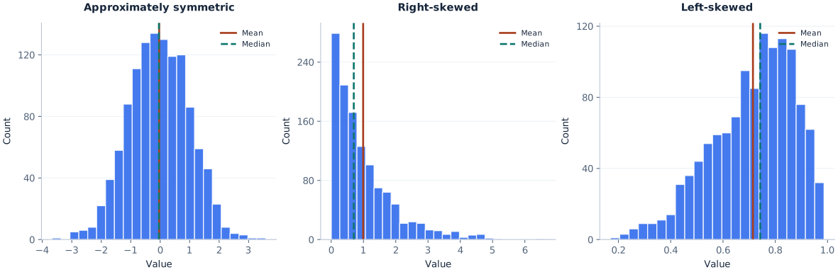
In these reproducible samples, the right-skewed mean is approximately 0.99 and median 0.70; the left-skewed mean is approximately 0.71 and median 0.74. Their order agrees with the usual tendency. Do not turn this into a law: mean > median is not the definition of right skew, and mean = median does not prove symmetry. Mean–median–mode inequalities should not be taught as guaranteed for all distributions.
Spread is a separate property. Two similarly shaped distributions can be narrow or wide; a single standard deviation describes part of this variation but not the full picture. See standard deviation explained for that calculation.
How Bin Width Changes Histogram Shape
A histogram does not display every observation at once. It groups measurements into intervals, so its apparent pattern depends on the chosen number of bins, their widths and where the first boundary begins. Too few bins can merge groups into a single broad mound. Too many can make sampling noise look like a collection of new peaks.
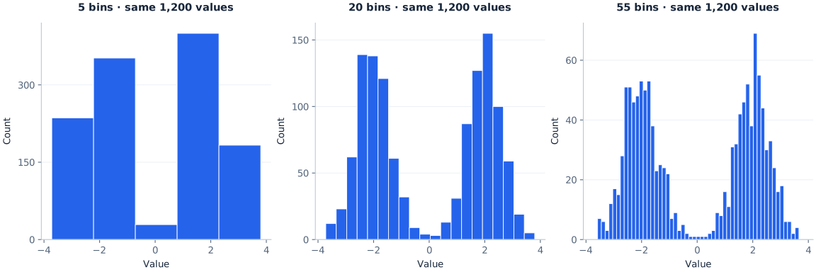
For a small dataset, even a moderate bin choice may be unstable. When comparing two histograms, changing boundaries can make a feature seem larger or smaller without changing the original records. Choose bins for faithful description, not to force the story you hoped to find.
Try the Bin Count Yourself
The demonstration below uses the same 1,200 bimodal observations as the illustration. Select a bin count and watch the distribution regroup. No observations are added or removed.
20 bins • 1,200 observations • identical input data
JavaScript is optional. The static three-panel figure above shows the same comparison.
Real analytical tools often offer automatic binning as a starting point, but there is no one correct bin count for every dataset. See the construction tutorial for manual and spreadsheet methods. This demonstration changes the number of equally sized bins; changing the start boundary can also change what seems prominent.
How Sample Size Affects Histogram Shape
With only a few dozen observations, a sample histogram can look ragged even when the underlying population is smooth and unimodal. With more observations, the picture may become more stable under sensible bin choices. More data cannot correct biased sampling or measurement problems, but they often reduce random fluctuations in the observed frequencies.
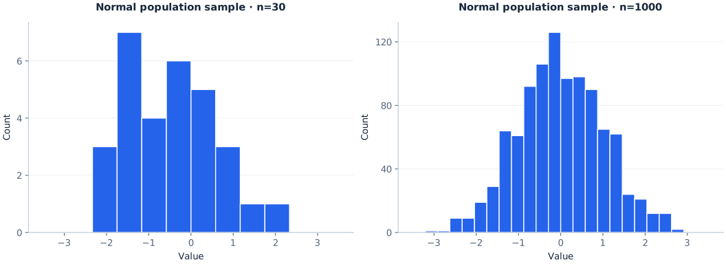
If a tiny histogram appears bimodal or uniform, describe what is visible without claiming the sample establishes the population shape. Recheck the pattern with more data if available, and ask whether the sampling method fairly represents the process being studied.
How to Compare Histogram Shapes Fairly
Before comparing groups, make sure the x-axes describe the same numerical variable and units. Use the same relevant horizontal range and compatible bin boundaries where possible. If sample sizes differ, raw counts can mislead: a group with twice as many observations may have bars roughly twice as high even with a similar distribution.
Relative frequency, percentage or suitably scaled density can help compare distributions of different sample sizes. With equal bin widths, switching counts to percentages changes the vertical scale but not the within-sample pattern. If widths differ, areas rather than raw bar heights must be interpreted carefully.
When group comparison matters more than the fine details of peaks, a box plot can summarize center and spread. When the variable is categorical, not numeric, read histogram versus bar graph. For chart selection generally, see how to choose the right chart type.
Example: Comparing Rainfall in Two Cities
Imagine two histograms of daily rainfall for City A and City B over the same year, drawn with the same bins and the same axis. A glance may show that both are right-skewed: most days have little or no rain and a few have heavy downpours. It may also show that City B's tail stretches much further. That is the main strength of a histogram for comparing data sets. It makes symmetry, skew, peaks and gaps visible at once.
Means, medians and standard deviations are not drawn on a plain histogram. You can only estimate them roughly from the bars, so calculate them separately, for example with the descriptive statistics calculator, when you need exact values. This is the reasoning behind a common textbook question: a histogram is useful for comparing the shapes of two data sets mainly because it makes their symmetry and skew easy to compare visually.
Histogram Shape vs Distribution Shape
The phrase “distribution shape” often refers to properties of the underlying values or the model believed to generate them. A histogram's appearance is an empirical, binned approximation of those properties. A probability density curve is instead a mathematical representation on a continuous scale. They can tell related stories, but they are not interchangeable.
This explains why a histogram may be approximately bell-shaped while a fitted model performs poorly in its tails, or why one conspicuous modal interval does not prove the raw values have a unique exact mode. Start with the visual description, then use additional data and analysis if you need a population-level conclusion.
Practice: Name the Histogram Shape
Read each description, name the shape in words using the layers above, then open the answer.
- Most bars are tall near the low end of the scale, and a thin run of short bars stretches toward high values.
Answer
Unimodal and right-skewed (positively skewed). The tail, not the peak, names the skew.
- Two mounds of similar height sit at equal distances from the middle, with low bars between them.
Answer
Approximately symmetric and bimodal. It is worth splitting the data by group.
- Every bar is within a few counts of its neighbors across the whole range.
Answer
Approximately uniform, and therefore roughly symmetric.
- The tallest bars are near the top of the scale, and frequencies thin out toward low values.
Answer
Left-skewed (negatively skewed).
- Bars alternate tall, short, tall, short across an otherwise smooth mound.
Answer
A comb pattern. Check the measurement rounding against the bin width.
- Frequencies are highest at both ends and lowest in the middle.
Answer
U-shaped.
- A smooth mound ends abruptly at two vertical walls with nothing beyond them.
Answer
Truncated (heart-cut). Ask whether the data were screened against limits before they were recorded.
Common Histogram Shape Mistakes
- Naming skew from the tall bars. The main cluster is not the naming rule. Find the longer tail and name its direction.
- Calling every symmetric display normal. Uniform-like and bimodal distributions may also be symmetric. Describe symmetry separately from the number of peaks.
- Declaring normality from a bell-shaped plot. Binned sample bars are not a formal distribution test. Use additional diagnostics when the assumption matters.
- Expecting uniform samples to be perfectly flat. Random samples fluctuate. Look for a broadly even pattern rather than identical rectangles.
- Claiming two peaks prove two populations. Peaks may arise from group mixtures, but also from binning and chance. Investigate possible explanations.
- Assuming the modal bin is the exact raw-data mode. The bin groups a range of values. Look at individual observations when an exact mode is meaningful.
- Interpreting an empty bin as an impossible range. It may be empty only in this sample or under these boundaries.
- Labeling a sparse far-end bar an outlier automatically. Inspect the original values and use context or a defensible rule.
- Comparing counts across different sample sizes. Consider relative frequencies and compatible axes.
- Describing shape from one arbitrary bin count. Check whether the overall interpretation holds when the grouping changes reasonably.
- Ignoring how the data were collected. Screening, rounding and lumping values into an “over” bin can create cliffs, combs and edge peaks that describe the recording process more than the variable.
- Using a histogram for a handful of possible values. For a rating scale or a die with only a few outcomes, a bar chart of each value is usually clearer.
See also AmriData's guide to data visualization mistakes, particularly when axis or chart choices distort the message.
Explore Histogram Shapes With AmriData's Histogram Maker
If you have your own numerical dataset, use the AmriData Histogram Maker to check its visible shape. Paste numbers separated by commas or line breaks, select an automatic or custom bin count, and generate the chart. Try another reasonable bin count if the first result seems unexpectedly flat or full of little peaks.
The current tool offers Sturges, square-root or custom bin counts, frequency or relative-frequency vertical axes, optional mean and median lines and PNG export. The standalone tool says its pasted values are processed in browser JavaScript; that statement concerns this tool, not every AmriData product. The tool changes bin count rather than exposing full manual control of exact bin edges, so use other plotting software when precisely matched boundaries are necessary.
Open Histogram Maker → You can also review the steps of exploratory data analysis to put your chart into a wider data-quality check.
Frequently Asked Questions About Histogram Shapes
What are the common histogram shapes?
Common descriptions include symmetric, bell-shaped (mound-shaped), approximately uniform, right-skewed, left-skewed, unimodal, bimodal and multimodal. Less common names include J-shaped, reverse J-shaped and U-shaped, and quality-control work adds plateau, comb, edge peak, truncated and dog food. They are not mutually exclusive: one chart can be symmetric and bimodal, or unimodal and skewed.
What are the 4 shapes of distribution in statistics?
Many introductory courses teach four basic shapes: symmetric (often bell-shaped), skewed right, skewed left and uniform. Others add bimodal as a fifth. The lists vary by textbook because symmetry, skew and the number of peaks are separate properties that can be combined.
How do you identify the shape of a histogram?
Check whether the two sides balance, look for the direction of any longer tail, count major peaks and note gaps or isolated regions. Test whether those features persist across sensible bin choices.
Is every bell-shaped histogram normally distributed?
No. “Bell-shaped” describes the visible pattern. A normal distribution is a specific probability model. A histogram alone cannot confirm that model, even when the sample bars resemble a bell.
What is a mound-shaped histogram?
A mound-shaped histogram has one rounded central peak with frequencies falling away on both sides. It is a looser name for a bell-like shape and does not imply a normal distribution.
Can a symmetric histogram have two peaks?
Yes. A bimodal distribution can be approximately symmetric if its two concentrations are balanced around the middle. Symmetry and the number of peaks describe different features.
What is the difference between a uniform and a symmetric histogram?
Symmetric means the two sides balance; uniform means the bars are broadly the same height with no clear peak. A uniform-like histogram is usually also symmetric, but a symmetric histogram can be bell-shaped, bimodal or U-shaped instead of flat.
Does a uniform histogram have equal-height bars?
Not necessarily. In a random sample from a uniform population, adjacent equal-width bins are expected to receive similar counts over the long run, but individual counts fluctuate.
Which way does a positively skewed histogram point?
Its longer tail extends to the right, toward larger numerical values. The tall bars may be clustered to the left. Positive skew is named for the tail direction.
Which way does a negatively skewed histogram point?
Its longer tail extends to the left, toward smaller numerical values. Negative skew is another term for left skew.
Can a histogram be unimodal and skewed?
Yes. “Unimodal” counts peaks and “skewed” describes asymmetry, so a histogram with one peak and a long right tail is unimodal and right-skewed.
What does a bimodal histogram tell you?
It shows two apparent concentrations or peaks. That may motivate checking groups or processes, but two peaks do not, by themselves, prove there are two populations.
What does a J-shaped histogram mean?
Frequencies rise steadily toward one edge of the range, like the letter J. It is an extreme skew, often found next to a hard limit. A reverse J-shaped histogram has its tallest bar at the low end instead.
What is a U-shaped histogram?
A U-shaped histogram has its tallest bars at both ends and its lowest bars in the middle, which means values gather at two extremes. Check the scale limits and whether two different groups are present.
What does a comb-shaped histogram mean?
Alternating tall and short bars usually point to rounding or instrument resolution that does not fit the bin width. Rebuilding the chart with a bin width that is a whole multiple of the measurement step often removes the comb.
Can changing histogram bins change the apparent shape?
Yes. Fewer bins may smooth over distinct clusters; more bins may create noisy local bumps. Bin width and the starting boundary affect the apparent pattern even though the observations are unchanged.
What is a bin in a histogram?
A bin is one of the numerical intervals the horizontal axis is divided into. Each bar's height shows how many observations, or what share of them, fall in that interval. See the frequency distribution table guide for how bins are built.
Why are histograms useful for comparing the shapes of two data sets?
Drawn on the same scale, two histograms make symmetry, skew, peaks and gaps easy to compare at a glance. Means, medians and standard deviations are not shown directly, so they are better compared with calculated statistics.
Does a higher mean than median always mean a histogram is right-skewed?
No. A mean above the median is common for many right-skewed distributions but is not a definition or a reliable universal test. Judge skew primarily from distributional asymmetry and the tail.
Does an isolated bar mean my dataset has outliers?
Not automatically. A sparse interval can flag values for review, but identifying potential outliers requires the raw observations, context and an appropriate method. The guide to finding outliers and the outlier calculator cover common rules.
Where can I learn how to draw these shapes from raw numbers?
Use AmriData's how to make a histogram tutorial for manually constructing bins and frequencies, or try the Histogram Maker.
Key Takeaways
- Describe histogram shapes in layers: symmetry or skew, number of peaks, and unusual features, alongside center and spread.
- A longer right tail signals right skew; a longer left tail signals left skew, regardless of where the tallest bars sit.
- Symmetry does not mean normality, and a bell-shaped sample cannot prove a normal population. Uniform, bimodal and U-shaped histograms can be symmetric too.
- One peak is unimodal, two suggest bimodality and more than two suggest multimodality; these impressions depend on binning and sample size.
- Quality-control names such as plateau, comb, edge peak, truncated and dog food usually point to how data were mixed, rounded, grouped or screened.
- Check raw data, sensible bin choices, sample size and context before drawing strong conclusions from gaps or sparse regions.
Histogram shapes are most useful when described cautiously and precisely. For more statistics lessons return to the Statistics category, or open the Histogram Maker to compare several binnings of your own values.
Related Statistics Guides and Tools
← Back to all Statistics articles
References and Data Notes
- NIST/SEMATECH e-Handbook: Histogram — descriptive interpretation, skewness, modality and follow-up analysis.
- NIST/SEMATECH e-Handbook: Histogram Interpretation, Skewed Left — skew direction and distribution asymmetry.
- NIST/SEMATECH e-Handbook: Symmetric and Bimodal — modality and possible explanations.
- ASQ: What Is a Histogram? — quality-control pattern names (plateau, edge peak, comb, truncated, dog food), adapted by ASQ from The Quality Toolbox.
- OpenStax: Histograms, Frequency Polygons, and Time Series Graphs — shape, center and spread.
Illustration methodology: the primary visual comparisons use reproducible synthetic random samples (seed 20261016; n = 1,200 per main shape), generated from normal, uniform, exponential, beta and separated normal-mixture models. The sample-size illustration independently uses seed 777 and sample sizes 30 and 1,000. The J-shaped, U-shaped and quality-control pattern illustrations use seed 20261113 and n = 1,200 each. They were generated from beta distributions, a five-group normal mixture, and normal samples that were rounded, lumped into an “over” bin, screened at fixed limits or combined with a small separate group. Source code and exact metadata are included with the downloadable assets. These are educational simulations, not measurements from AmriData customers.